Chapter 8 Bayesian phylogenetics
Let’s take stock of what we have covered so far. We introduced models, and how to simulate data with them. We then explored how to use models to calculate the likelihood—the probability of the observed data given the topology, branch lengths, model parameters, and model. We used likelihood as an optimality criterion in heuristic searches to find the maximum likelihood (ML) phylogeny. We introduced the methods to calculate the frequency of branches on a focal topology, like the ML topology, in a sample of phylogenies. We showed how to generate a sample of phylogenies by running ML searches on bootstrapped matrices, and used this to calculate bootstrap support for each branch in the ML phylogeny.
ML and bootstraps are widely used and are a critical foundation for many phylogenetic analyses. There are, however, a few things about analysis frameworks based on optimality criteria, ML, and bootstraps that are not ideal:
Whenever we apply an optimality criterion, such as ML or parsimony, to identify the “best” phylogeny, that doesn’t tell us anything about how much better this optimal phylogeny is than other hypotheses. If it is the best phylogeny by far, then this single phylogeny tells us a lot about the phylogenetic information in our analysis. If, however, there are multiple phylogenies that are almost as good as the best one, as is often the case, then we would need to know about these others as well to have a good understanding of what hypotheses are consistent with our data.
Likelihood is the probability of the data given the phylogenetic hypothesis. The probability of the data under the ML hypothesis will be exceptionally low, often far less than one in a million, since the ML hypothesis could generate many other datasets as well. This is because we are evaluating the probability of the data given the hypothesis, but often what we really want to know is the probability of the hypothesis given the data. The two are quite different, but are related. It would be nice to be more explicit about that relationship.
Bootstraps are a convenient way to generate a sample of phylogenies, but their statistical interpretation is not clear. The frequencies of bootstrap supports don’t correspond in a clear way to probabilities of our hypothesis, but instead tell us something about how frequently features of the phylogeny are supported when we resample the data. In practice it turns out this is a good proxy for phylogenetic support, but it would be nice to have support values that have a more explicit statistical interpretation.
All analyses include a variety of tradeoffs, and the issues listed above are often mitigated by the multiple upsides of an ML bootstrap analysis framework. It also greatly helps that there are decades of experience with ML analyses that help contextualize and interpret ML bootstrap results. This work has produced ML methods and software packages that are highly optimized for computational efficiency, enabling the routine application of these approaches to very large datasets.
Another analysis framework, Bayesian statistics, directly addresses all of the issues listed above (Yang and Rannala 1997; Holder and Lewis 2003; Huelsenbeck and Ronquist 2001; Larget and Simon 1999; Chen et al. 2014). Rather than focus on a single “best” topology, it provides a set of hypotheses consistent with the data. The frequencies of these hypotheses in the sample are the expected probabilities of the hypotheses given the data. These frequencies have a clear probabilistic interpretation, unlike the bootstrap support values. Bayesian statistics and likelihood have deep mathematical connections, so we will be able to build directly on the foundation established in previous chapters.
8.1 Bayesian statistics
Bayesian statistics is much older than many other domains of statistics, but has recently seen a surge in use as computational and methodological advances allow it to be applied more effectively to a wider range of problems. The basic intuition is that our understanding of the world is not drawn from the data alone. Instead, the data are used to update our prior understanding of the world. This updated understanding is referred to as the posterior. There are many excellent introductions to Bayesian statistics, so I will not provide a full derivation here. If you would like more of a background, please consult Appendix A.2.
Bayes’ theorem establishes the following relationships:
\[\begin{equation} P(H|D) = \frac{P(D|H)P(H)}{P(D)} \tag{8.1} \end{equation}\]
\(P(H|D)\), read as “the probability of the hypothesis given the data”, is the posterior probability of a given hypothesis. It takes into account prior expectations and new insight from the data. This posterior probability is what we are trying to estimate. We have already seen \(P(D|H)\), read as “the probability of the data given the hypothesis”. This is the likelihood, and from previous chapters we know how to calculate it. \(P(H)\) is the prior probability of the hypothesis, our world view before we collected data. \(P(D)\) is the probability of the data averaged over all hypotheses, each weighted by its prior probability. It is not a prior belief about the data in the way that \(P(H)\) is a prior belief about the hypothesis; it is the normalizing constant that ensures the posterior sums to one across all hypotheses.
Let’s plug in a few numbers to get some intuition for the behavior of Bayes’ theorem. First, consider the case where \(P(H)=0\), i.e., you assign a prior probability of \(0\) to the hypothesis. The posterior probability, \(P(H|D)\), will then also be \(0\). This shows that if you believe ahead of collecting data that the hypothesis is absolutely impossible, no amount of data can change your mind and your updated hypothesis, the posterior, will also be \(0\).
Second, let’s consider the case where the data are just as likely under the hypothesis as they are under other hypotheses. This would be like having a medical test for a specific condition where the test was so bad that the data (test result) didn’t depend in any way on the hypothesis (the presence of the condition). For example, the test returns a positive 10% of the time regardless of whether you have the condition or not. In that situation, \(P(D|H)=P(D)\). Since \(P(D|H)\) is in the numerator and \(P(D)\) is in the denominator, they cancel out. That leaves \(P(H|D)=P(H)\)—the posterior probability of the hypothesis is the same as the prior on the hypothesis. The data didn’t change our understanding of the hypothesis at all. This is the behavior we want when the data have no information relevant to the hypothesis.
Third, consider a case where the data are perfect indicators of the hypothesis. You get a specific pattern in the data whenever, and only when, the hypothesis is true. Because the hypothesis and data are perfectly linked, \(P(D)=P(H)\), and the priors cancel out. In this case, \(P(H|D)=P(D|H)\), i.e., the posterior becomes equal to the likelihood. This never happens in phylogenetic inference, since any given phylogeny could always generate multiple sequences at the tips. But it is generally the case that as the data become more informative, the priors have less impact on the posterior.
8.2 Bayesian phylogenetic inference
To calculate the posterior probability of a phylogenetic hypothesis, we need to address all the terms on the right side of Equation (8.1). We already know how to calculate \(P(D|H)\), the likelihood. What about \(P(H)\) and \(P(D)\)? There are a variety of practical approaches to \(P(H)\) that have been shown to work well in the context of phylogenetics. These include a uniform prior on topologies, under which all distinct topologies are assigned equal prior probability. Branch length priors are often modeled with an exponential distribution.
What, then, about \(P(D)\)? Calculating it requires integrating the probability of generating these particular character data (e.g., nucleotide sequences observed at the tips) across all possible topologies and branch lengths, weighted by their priors. That would be prohibitively computationally expensive to actually do. So we won’t.
Instead, we will forego calculating \(P(D)\) by approximating the posterior with Markov Chain Monte Carlo (MCMC) sampling (Metropolis et al. 1953; Hastings 1970). MCMC is a widely used method to approximate probability distributions that are too complex to calculate analytically. MCMC is implemented by proposing a series of hypotheses that are either rejected or accepted based on a specially formulated acceptance ratio \(R\) and criteria for evaluating it, such that the accepted hypotheses form a sample that is drawn from the distribution of interest. In our case, that distribution of interest is the posterior distribution.
Consider the current hypothesis to be \(H\), and the newly proposed hypothesis \(H^*\). We calculate this acceptance ratio as the ratio of the posterior probability of \(H^*\) to the posterior probability of \(H\):
\[\begin{equation} R = \frac{P(D|H^*)P(H^*)}{P(D)} \frac{P(D)}{P(D|H)P(H)} = \frac{P(D|H^*)P(H^*)}{P(D|H)P(H)} \tag{8.2} \end{equation}\]
Because \(P(D)\) doesn’t depend on the hypothesis under consideration, it is the same in both posteriors. Because we are considering a ratio of posteriors, it cancels out. We don’t need to calculate it to derive \(R\).
This form assumes the proposal mechanism is symmetric—that proposing \(H^*\) from \(H\) is as probable as the reverse. When it is not, an additional proposal ratio corrects for the asymmetry; we omit it here for simplicity.
The “Markov Chain” in MCMC alludes to the fact that MCMC is a series of repeated events that depend only on the previous step. Each repeated cycle of events, also known as a generation, proceeds as follows:
- We have hypothesis \(H\).
- We propose a new hypothesis \(H^*\) by modifying \(H\).
- We calculate \(R\) according to Equation (8.2).
- If \(R \geq 1\), we accept \(H^*\). Otherwise, we accept \(H^*\) with probability \(R\), and retain \(H\) if it is not accepted.
- The result of the step above is added to the posterior sample, and becomes \(H\) for the next iteration of the cycle.
MCMC produces a sample of model parameters and topologies with branch lengths. This sample is an approximation of the posterior distribution of these entities. We can summarize the topologies in this posterior sample in the same way we did for bootstraps, with branch frequencies. Unlike bootstraps, though, the frequency of a branch in this distribution has a clear statistical interpretation. It is an approximation of the posterior probability of that branch, i.e., the probability of the branch given the data and our priors. The branch lengths and model parameters form continuous probability distributions. We can summarize these in a variety of ways, for example by taking the mean for each.
8.3 Bayesian phylogenetic inference in practice
There are a variety of practical considerations to implementing a Bayesian phylogenetic analysis with MCMC. These analyses are carried out with widely used software packages such as MrBayes (Huelsenbeck and Ronquist 2001; Ronquist et al. 2012) and BEAST (Drummond and Rambaut 2007). The practical considerations include:
- Selecting the appropriate model. Many of the same considerations we reviewed in the context of likelihood apply here.
- Selecting appropriate priors on topology, branch length, and model parameters.
- Devising an appropriate hypothesis proposal mechanism. The scale of the proposals does not change the distribution the chain is sampling from—with a correct Metropolis-Hastings implementation the chain converges to the same posterior regardless of proposal scale. What the proposal scale affects is efficiency: how quickly the chain explores the posterior, and therefore how well a run of finite length approximates it. If the proposed hypothesis \(H^*\) is usually far from \(H\), most proposals land in regions of low posterior probability and are rejected, so the chain stays in place for long stretches and moves slowly. If the proposals are instead very small, most are accepted but each step barely moves, so the chain drifts slowly and successive samples are highly autocorrelated. Either extreme mixes poorly: successive samples carry little new information, the effective sample size is low, and a run of a given length gives a noisier, less reliable approximation of the posterior. In the worst case a finite run may not have had time to move between well-separated regions of high probability at all, so it misses part of the posterior even though the target distribution it would eventually sample is correct. Good proposals strike a balance, and there are several approaches to tuning them, including searches with multiple MCMC chains that take different step sizes.
- The very early samples in the chain are not a good estimate of the posterior distribution, because the initial \(H\) is not necessarily close to a peak in the posterior. The initial samples before MCMC settles into a stable distribution are therefore discarded as part of a “burn-in” phase.
- Knowing when enough generations have been sampled to adequately approximate the posterior distribution. This is often evaluated by running multiple independent MCMC analyses and stopping them if and when they have converged on similar distributions.
The ability to specify a prior can be a great advantage of Bayesian analyses. A prior is an explicit, principled way to incorporate prior knowledge into a new analysis. For example, if you are very confident that a particular clade exists based on external evidence, you could design a topology prior that favors topologies that include that clade over topologies that don’t. If you have external information about model parameters, you could set a prior that constrains these parameters. These are cases of what are called informative priors—they are nonuniform, and intentionally constrain results based on external information. In many cases, though, investigators use relatively diffuse, or vague, priors that spread probability broadly across hypotheses rather than concentrating it. If you are ever concerned about the impact of your priors on your posteriors, you can run your analysis without any data—the posterior will then be determined entirely by the prior. This gives you a good understanding of the impact of your prior on the posterior, and by comparing this empty analysis to an analysis with data you can get a good sense of the impact of your data on the posterior.
Bayesian phylogenetic software stores samples of the run at regular intervals, for example every hundred generations (where a generation is a single MCMC proposal). Typically, there are two output files, a tree file and a trace file. The tree file has one line per sample, each with a tree in Newick format. The trace file also has one line per sample. There are multiple columns, each with a model parameter or run statistic. It is called a trace file because you can plot each of these columns to trace the progress of the MCMC run.
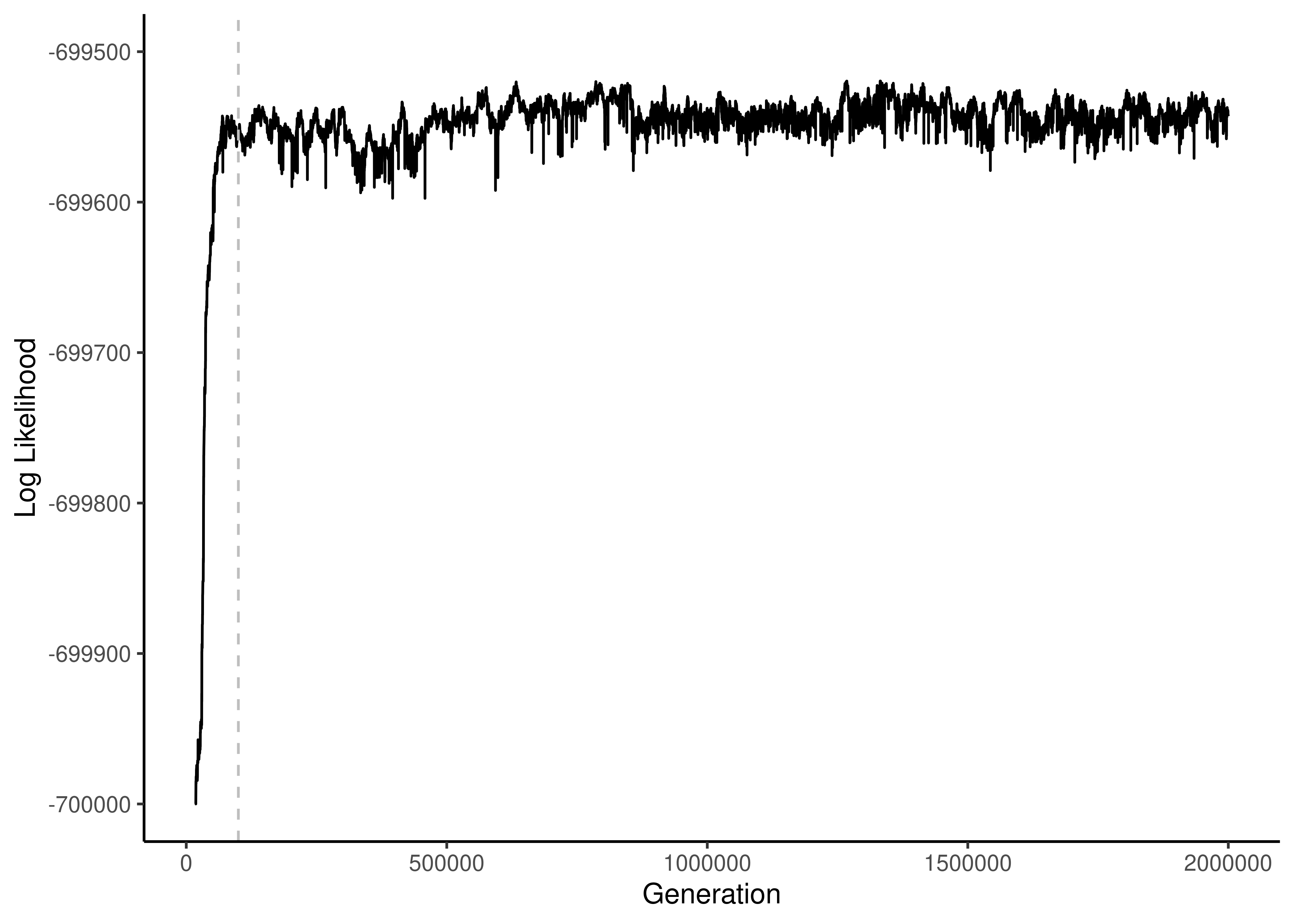
Figure 8.1: Plot of log likelihood trace for a Bayesian analysis. A burn-in of 100,000 generations is indicated with a dashed vertical line.
Investigators should at minimum examine the trace of log likelihood (Figure 8.1). There are a few things to look for. First, an appropriate burn-in should be identified. This is the number of generations at the start of the run that are discarded as the MCMC chain settles into the sampling process. During the burn-in, the log likelihood rapidly climbs as the chain moves toward higher likelihood regions of tree and model space. In the example provided here, the chain appears to have moved past this initial climb after roughly 100,000 generations. Second, the investigator should examine the post-burn-in sampling process to make sure it looks well mixed. It should appear noisy, as it does here, indicating that trees and model parameters with a range of likelihoods are sampled, and it should not show sudden major jumps or longer-term trends, which can indicate inadequate sampling.
A noisy, trend-free log likelihood trace is necessary but not sufficient evidence that a run is sampling the posterior well. A chain can look perfectly stationary in log likelihood while remaining stuck in one region of tree space, or while individual parameters remain poorly sampled, and the log likelihood alone cannot reveal this. Nor does choosing a burn-in establish convergence: discarding the initial samples only removes the early transient before the chain reached its current region. If a chain has not mixed or converged, no choice of burn-in can repair it.
Other diagnostics are available to assess whether a run has adequately sampled the posterior. These include examining the traces of individual model parameters and calculating the effective sample size (ESS) for each parameter. The ESS estimates how many effectively independent samples the autocorrelated chain provides for a given parameter; a low ESS (a common rule of thumb flags values below a few hundred) signals high autocorrelation and poor mixing, and calls for a longer run or better proposals.
Once the trace file has been examined, the investigator turns to the tree file. All pre-burn-in trees are discarded. You then pick a focal tree, which could be the maximum likelihood tree or consensus of the post-burn-in Bayesian trees. The frequency of each edge in the focal tree is then calculated from the set of post-burn-in trees and recorded as the posterior probability of that edge. These are then plotted onto the tree, often along with the maximum likelihood bootstrap scores.
8.4 Resources
- A video introduction to Bayes’ theorem: https://www.youtube.com/watch?v=HZGCoVF3YvM
- The excellent MCMC robots by Paul Lewis: https://plewis.github.io/applets/mcmc-robot/