Chapter 4 Inferring phylogenies from data
In the previous chapter we built modeling machinery that allowed us to specify a rate matrix \(\mathbf{Q}\) (Equation (3.8)), and from that derive the matrix \(\mathbf{P}(t)\) (Equation (3.7)) that gives the probability of a particular end state given the starting state and the branch length \(t\). We used \(\mathbf{P}(t)\) in a generative context, to simulate the evolution of a DNA sequence along the branches of a phylogeny.
We will now turn to using the same statistical framework for what may initially seem to be a very different task – phylogenetic inference, where we infer the topology and branch lengths of a phylogeny from character data (DNA sequences, in this case). But these tasks are similar conceptually. The basic intuition is that you can infer a phylogeny by looking for the topology and branch lengths that are most likely to generate the observed data (Felsenstein 1981).
This relationship between simulation and inference is widely used in a variety of fields. The probability of the observed data given a hypothesis is referred to as the Likelihood. Searching for the most likely hypothesis is referred to as Maximum Likelihood (ML).
4.1 Probability of a single history
We will consider the toy phylogeny, along with its tip states, shown in Figure 4.1.
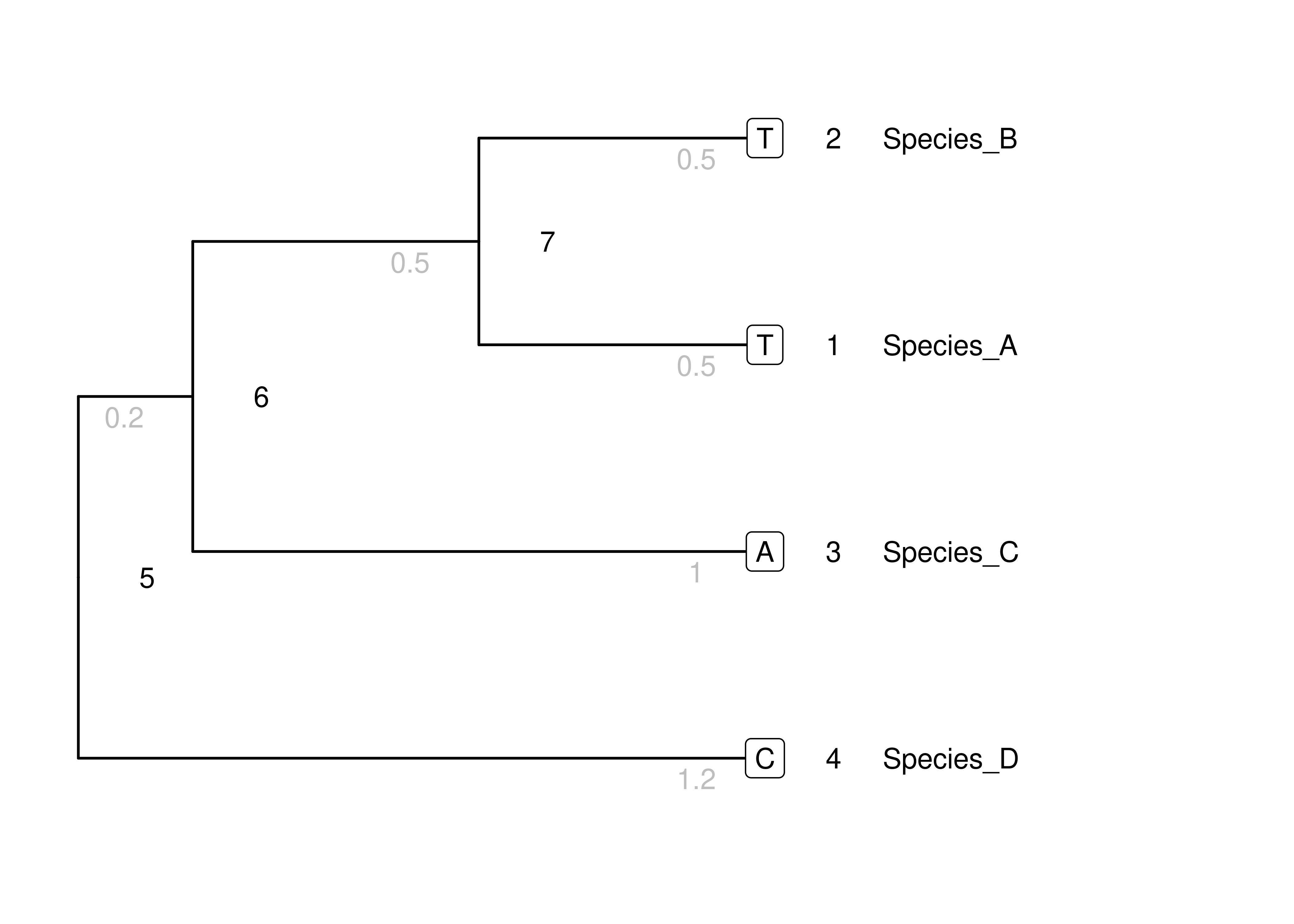
Figure 4.1: The toy phylogeny we will use to examine inference. Node numbers are in black. Branch lengths are gray numbers below branches. Tip node states are within boxes.
We will start be calculating the probability of a single history of evolution for a single site on a single phylogeny with specified topology and branch lengths. This history is a full set of states at all nodes. These are added to the toy phylogeny in Figure 4.2. This isn’t a history we have any particular reason to believe, it is just one possible history of states randomly chosen from all the possible histories.
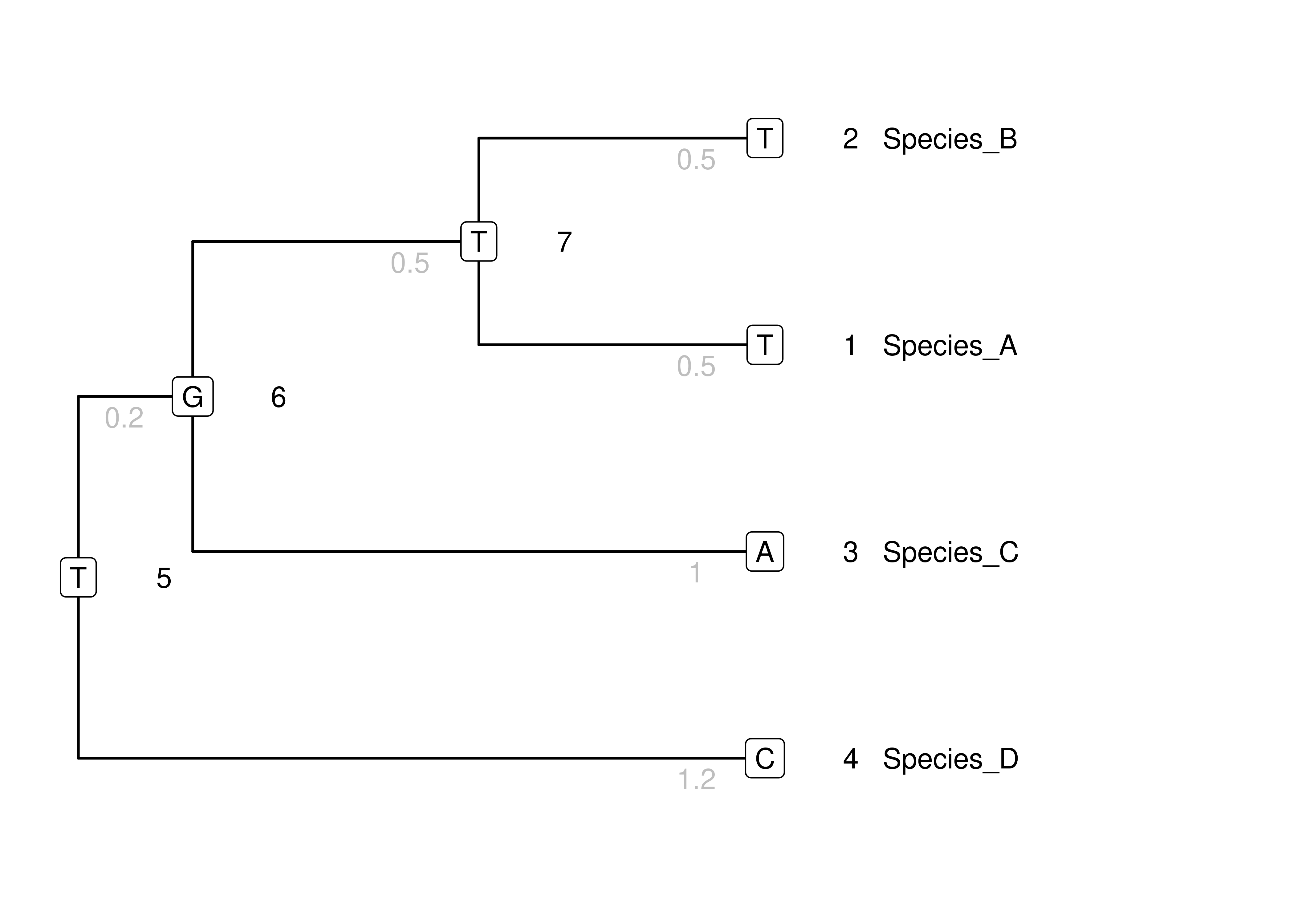
Figure 4.2: The same toy tree as above, but with arbitrary internal node states (in boxes).
Our goal now is to calculate the probability of each observed change. Recall that the matrix that contains these probabilities, given a starting state (rows), ending state (columns), and branch length \(t\), is given by:
\[\begin{equation} \mathbf{P}\left(t\right) = e^{\mathbf{Q} t} \tag{4.1} \end{equation}\]
Where \(\mathbf{Q}\) is the rate matrix. Let’s plug some numbers in using the model we specified in the previous chapter. We don’t have any specific reason to use this model on this tree, we are just sticking with it since we already built it.
Here is the relative rate matrix \(\mathbf{R}\):
##     A   C   G   T
## A 0.0 0.5 2.0 0.5
## C 0.5 0.0 0.5 2.0
## G 2.0 0.5 0.0 0.5
## T 0.5 2.0 0.5 0.0
The equilibrium frequencies \(\mathbf{\Pi}\):
##       A     C     G     T
## A 0.295 0.000 0.000 0.000
## C 0.000 0.205 0.000 0.000
## G 0.000 0.000 0.205 0.000
## T 0.000 0.000 0.000 0.295
And their product \(\mathbf{Q}\), with the diagonal adjusted so that rows sum to 0:
##         A       C       G       T
## A -0.6600  0.1025  0.4100  0.1475
## C  0.1475 -0.8400  0.1025  0.5900
## G  0.5900  0.1025 -0.8400  0.1475
## T  0.1475  0.4100  0.1025 -0.6600
For each branch, we can now use \(\mathbf{P}(t)\) to calculate the probability of a change from the start state at the parent node to the end state at the child node, given the branch length \(t\). The results are shown in Figure 4.3.
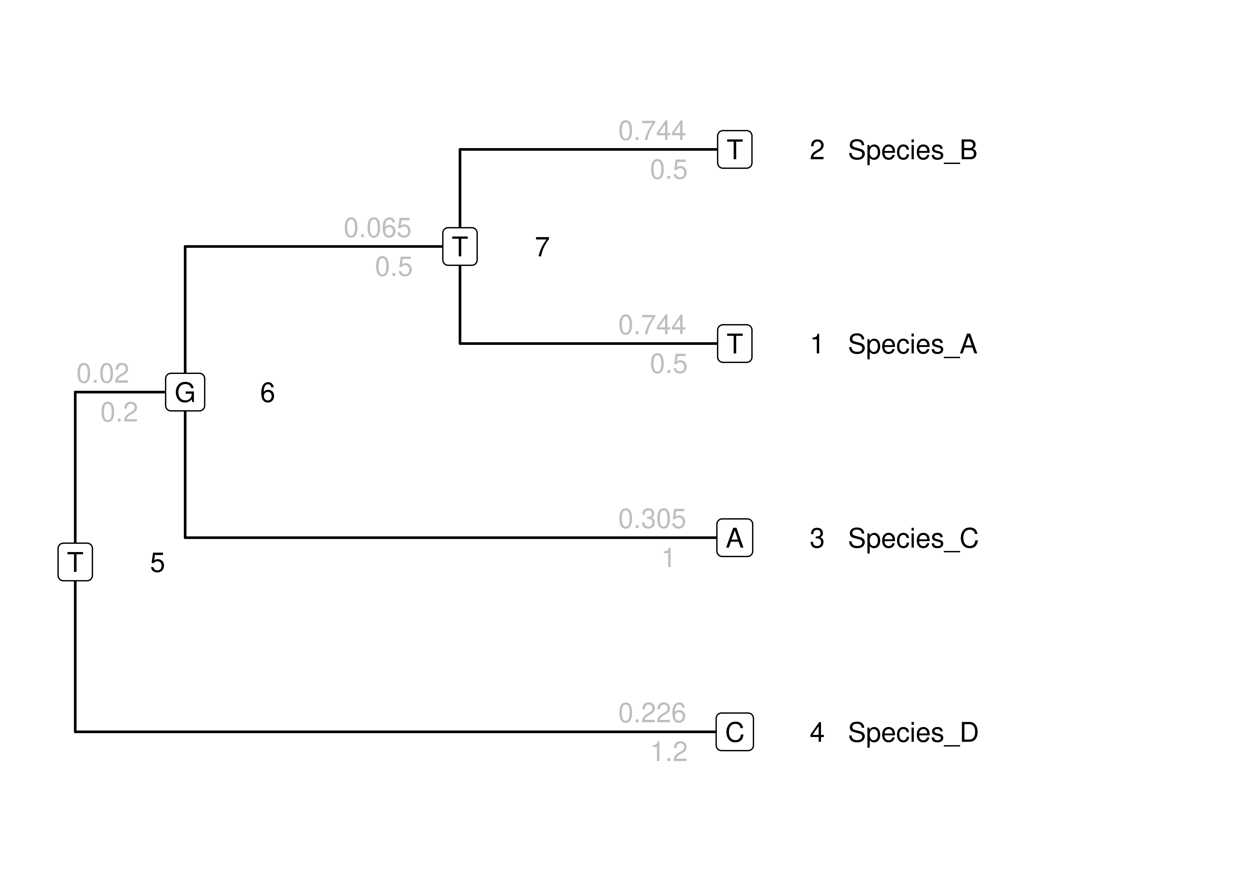
Figure 4.3: The same toy tree as above, but with probabilities of the specific change along each branch above each branch (in gray).
Now that we have the probabilities of each of these changes, we can calculate the joint probability of all these changes. When we want to calculate the joint probability of multiple independent events, we take the product of the probability of each specific event. For example, the probability of rolling a 4 on a fair die is \(1/6\). The probability of rolling two 4s on two fair dice is \(1/6\times1/6=1/36\). So we can take the product of all the probabilities to calculate the joint probability of all of these events happening. We can think of the probabilities of specific changes along each branch as the probabilities of the state at each child node given the state at the parent node.
| node | probability |
|---|---|
| 1 | 0.7442034 |
| 2 | 0.7442034 |
| 3 | 0.3048887 |
| 4 | 0.2260230 |
| 5 | NA |
| 6 | 0.0195083 |
| 7 | 0.0652538 |
Note, though, that the probability for node 5, the root node, is missing. This makes sense since the root is not the child of any branch, and we calculated the probabilities based on changes along branches. We will therefore assess the probability of the root node state according to \(\mathbf{\Pi}\), the equilibrium frequencies. This is the same approach we took when simulating data on a tree. When we fill that in our full set of probabilities is:
| node | probability |
|---|---|
| 1 | 0.7442034 |
| 2 | 0.7442034 |
| 3 | 0.3048887 |
| 4 | 0.2260230 |
| 5 | 0.2950000 |
| 6 | 0.0195083 |
| 7 | 0.0652538 |
The joint probability of all these states can now be calculated as the product of each state. This comes out to \(1.4332602\times 10^{-5}\). There are multiple ways to think about this probability. One is from a frequentist perspective. If we were to simulate character states on this tree, we would expect this full set of character states to occur at a frequency of \(14.3\) times out of a million simulations.
Here we use much of the same machinery as in the previous chapter, but toward a slightly different end. Rather than use the probability distributions to generate nucleotides in a simulation, we instead calculated the probability of a particular set of nucleotides. These may have seemed like very different tasks at first blush, but as you can now see their mathematical implementation shares many features.
4.2 Probability of multiple histories
Above we considered the joint probability of a specific set of nucleotide states at all nodes, including both tip nodes and internal nodes. Usually, though, we don’t know the internal node states. We don’t even know what internal nodes exist, which is why we are trying to infer the phylogeny! Instead we have observed states that we got by sequencing organisms at the tips. We want to clamp these tip states and assess their probability on a particular tree (with branch lengths) under the model. This probability is independent of a specific history of internal node states.
If we aren’t clamping the internal node states as well, how can we calculate the probability of just the tip node states? The key is to consider all possible internal states. Each configuration of internal node states represents one possible history that gave rise to the observed tip states. We can sum the probabilities of each of these different ways to get the tip states to find the probability of the tip states over all possible histories. We are summing the probabilities because these are mutually exclusive histories that could give rise to the observed data. For example, if we want to find the probability of getting a total of seven when rolling two dice, we need to add up the probability of each way to get seven (1+6 or 2+5 or 3+4 or … 6+1). This is different from when we multiplied probabilities to find the joint probabilities of multiple events occurring together (e.g., the probability of rolling a 4 and another 4).
This is a small tree, with only 3 internal nodes that can each have 4 states. This gives \(4^3=64\) possible histories. That is small enough to list them out below. I also include the probability of each specific history, calculated as I did above (the example above corresponds to row 60 here).
| n1 | n2 | n3 | n4 | n5 | n6 | n7 | probability |
|---|---|---|---|---|---|---|---|
| T | T | A | C | A | A | A | 0.0000451 |
| T | T | A | C | C | A | A | 0.0000048 |
| T | T | A | C | G | A | A | 0.0000036 |
| T | T | A | C | T | A | A | 0.0000035 |
| T | T | A | C | A | C | A | 0.0000000 |
| T | T | A | C | C | C | A | 0.0000025 |
| T | T | A | C | G | C | A | 0.0000000 |
| T | T | A | C | T | C | A | 0.0000002 |
| T | T | A | C | A | G | A | 0.0000005 |
| T | T | A | C | C | G | A | 0.0000005 |
| T | T | A | C | G | G | A | 0.0000044 |
| T | T | A | C | T | G | A | 0.0000004 |
| T | T | A | C | A | T | A | 0.0000000 |
| T | T | A | C | C | T | A | 0.0000003 |
| T | T | A | C | G | T | A | 0.0000000 |
| T | T | A | C | T | T | A | 0.0000019 |
| T | T | A | C | A | A | C | 0.0000282 |
| T | T | A | C | C | A | C | 0.0000030 |
| T | T | A | C | G | A | C | 0.0000023 |
| T | T | A | C | T | A | C | 0.0000022 |
| T | T | A | C | A | C | C | 0.0000018 |
| T | T | A | C | C | C | C | 0.0002699 |
| T | T | A | C | G | C | C | 0.0000013 |
| T | T | A | C | T | C | C | 0.0000164 |
| T | T | A | C | A | G | C | 0.0000012 |
| T | T | A | C | C | G | C | 0.0000011 |
| T | T | A | C | G | G | C | 0.0000097 |
| T | T | A | C | T | G | C | 0.0000008 |
| T | T | A | C | A | T | C | 0.0000006 |
| T | T | A | C | C | T | C | 0.0000069 |
| T | T | A | C | G | T | C | 0.0000004 |
| T | T | A | C | T | T | C | 0.0000432 |
| T | T | A | C | A | A | G | 0.0000088 |
| T | T | A | C | C | A | G | 0.0000009 |
| T | T | A | C | G | A | G | 0.0000007 |
| T | T | A | C | T | A | G | 0.0000007 |
| T | T | A | C | A | C | G | 0.0000000 |
| T | T | A | C | C | C | G | 0.0000018 |
| T | T | A | C | G | C | G | 0.0000000 |
| T | T | A | C | T | C | G | 0.0000001 |
| T | T | A | C | A | G | G | 0.0000017 |
| T | T | A | C | C | G | G | 0.0000016 |
| T | T | A | C | G | G | G | 0.0000142 |
| T | T | A | C | T | G | G | 0.0000011 |
| T | T | A | C | A | T | G | 0.0000000 |
| T | T | A | C | C | T | G | 0.0000002 |
| T | T | A | C | G | T | G | 0.0000000 |
| T | T | A | C | T | T | G | 0.0000013 |
| T | T | A | C | A | A | T | 0.0005139 |
| T | T | A | C | C | A | T | 0.0000552 |
| T | T | A | C | G | A | T | 0.0000415 |
| T | T | A | C | T | A | T | 0.0000400 |
| T | T | A | C | A | C | T | 0.0000071 |
| T | T | A | C | C | C | T | 0.0010512 |
| T | T | A | C | G | C | T | 0.0000050 |
| T | T | A | C | T | C | T | 0.0000638 |
| T | T | A | C | A | G | T | 0.0000214 |
| T | T | A | C | C | G | T | 0.0000198 |
| T | T | A | C | G | G | T | 0.0001776 |
| T | T | A | C | T | G | T | 0.0000143 |
| T | T | A | C | A | T | T | 0.0000366 |
| T | T | A | C | C | T | T | 0.0004512 |
| T | T | A | C | G | T | T | 0.0000255 |
| T | T | A | C | T | T | T | 0.0028111 |
Note that I listed the states for all the nodes, including nodes 1-4, which are clamped. It is the last three internal nodes (n5-n7) that have variable states. The probabilities for each specific history range quite widely, from \(8.2902428\times 10^{-9}\) to \(0.0028111\).
The sum of the probabilities for each of these different histories for n5-n7 that give rise to the observed clamped states for tip nodes n1-n4 is \(0.0058252\). This probability of the data given a particular hypothesis (the topology, branch lengths, model, and model parameters) is the likelihood.
4.3 Log likelihood
The likelihood of these data on this phylogeny, \(0.0058252\), is not a big number. And this is a very small tree. As trees get larger there are many more probabilities we need to multiply, so the products get even smaller. The joint probabilities, in fact, get so small that computers have trouble storing them efficiently. Rather than store and manipulate the small probabilities directly, most tools take the natural logs of the probabilities, \(ln(p)\). The log likelihood for this phylogeny is \(-5.1455597\). Taking the log transforms probabilities to a numerical representation that is easier to work with. It also has the added value of making calculations of joint probability simpler. Given the relationship between the log of products of variables and the sum of logs of each value:
\[\begin{equation} ln(a)+ln(b) = ln(ab) \tag{4.2} \end{equation}\]
We can calculate joint log probabilities as sums of log probabilities for each event, rather than as the log of products of the probabilities. You will almost always see log likelihoods, rather than just likelihoods, published in the literature. Note that because likelihoods are probabilities and therefore range from 0–1, the log likelihoods will range from \(-\infty\) (for probabilities very close to 0) to \(0\) (for probabilities close to 1). Since likelihoods tend to be small, they end up as log likelihoods that are negative numbers with large absolute values.
4.4 Likelihood for multiple sites
The machinery above gives us everything we need to calculate the log likelihood of a specific pattern of nucleotides across tips for a single site in a DNA sequence. We now need to expand this model from a single site to multiple sites within a gene or even across whole genomes.
This comes down to more of the same. We do everything we did above for each site, and then sum the log likelihoods across sites. This gives us the joint probability of observing the data seen across tips for each site in the DNA sequence. This joint probability for all sites will be much smaller than the probability for each individual site.
4.5 Maximum likelihood
At this point we can calculate the log likelihood for specified phylogenies, models, and DNA sequences. But we set out to do phylogenetic inference, where we estimate phylogenies from sequences at tips. How do we get there from here? Once we can calculate the likelihood of a given phylogeny, we can calculate the likelihood of any phylogeny. We can then search for the phylogeny with the maximum likelihood (and, of course, maximum log likelihood).
The small toy phylogeny considered here (Figure 4.1) has four tip nodes. By reference to Equation (2.1), we can see that there are 15 possible topologies. For each, we can optimize the branch lengths to find the maximum likelihood for the topology. This is an iterative process, where each branch length is progressively refined until no change increases the likelihood. This excellent interactive visualization allows you to manually optimize branch lengths on a small phylogeny. Then we pick the topology with the maximum likelihood. This requires a very large number of calculations, but is doable for every possible topology.
Things change very quickly, though, as trees grow in size. Beyond about 15 tips there are so many possible topologies that it is impossible to calculate the likelihood for every topology using existing computer hardware and software. That means it is necessary to use heuristics - to modify the tree you have until you can do no better. This is like hill climbing. You calculate the likelihood of a tree and then modify it. If the likelihood is higher, you keep it, if it is worse, you discard it.
This might sound simple, but it isn’t. One challenge is that you can get trapped on a local maximum and mistake it for the best phylogeny, when in fact there are other phylogenies with very different topologies that are much better but not locally accessible. There is extraordinary craft that goes into building tools that are able to efficiently climb these likelihood surfaces without getting trapped in local maxima.
Optimization of calculations becomes very important. For example, it isn’t necessary to recalculate all values on each new topology, since some of the calculations from previous topologies remain relevant (Felsenstein 1981).
4.6 Optimality criteria
Here we used likelihood as an optimality criterion to search over treespace, the set of all possible phylogenies, to find the phylogeny that maximizes the criterion. There are other optimality criteria that are used in phylogenetic inference. These include parsimony. In parsimony, the minimum number of changes along branches needed to explain the data at the tips is used as the criterion to evaluate each topology. Optimization proceeds by attempting to identify the topology that requires the fewest changes. This requires far less computational power than likelihood, so searches are faster.
Under some conditions parsimony and likelihood will recover similar topologies, but often they do not. This is because they are doing different things that under many conditions lead to different results (Steel and Penny 2000). For example, we do not always expect the simplest possible explanation for a given pattern to be the best explanation. If a character has a high rate of evolutionary change, then we expect many changes on a tree rather than the fewest possible. This is accommodated in a likelihood framework.