Chapter 6 Evaluation
6.1 Model evaluation
We have examined models of DNA evolution in simulation and inference, but not yet how to select a model. Given a dataset, consisting of aligned DNA sequences for a set of taxa that correspond to tips on a phylogeny, how do you decide which model to use?
6.1.1 Model structure
Each model parameter can be treated in one of three ways (Hohna et al. 2014):
Constant. The parameter is clamped to a specific value before the analysis and is not free to vary.
Stochastic. The parameter is free to vary in the analysis. This allows the value to be estimated from the data as part of the inference process.
Deterministic. The parameter value depends on the values of other parameters according to specified mathematical relationships. Their values can vary, but are determined by the value of other parameters and cannot be set independently from them.
The most widely used DNA sequence evolution models include the General Time Reversible model and its derivatives (Section 3.4). The GTR model has 11 parameters (Figure 6.1). These include the global rate \(\mu\) used to tune the overall rate of evolution. Next come the relative rate parameters \(a,b,c,d,e,f\) that modify the rates of change between particular nucleotide states, so that they can differ from each other. For example, if a=0.5 and b=2, then the rate of changes between C and A occur at a rate four times higher than changes between A and G. Finally we have the equilibrium frequencies \(\pi_A,\pi_C,\pi_G,\pi_T\).
These parameters are treated as follows in the GTR model (Figure 6.1):
\(\mu\) is constant. With \(\mu=1\), the branch lengths are in units of expected evolutionary change.
The six rate parameters are constrained such that \(a+b+c+d+e+f=6\). If they were all free to vary, then values that have a sum other than 6 would lead to changes in the global rate rather than the relative rates. Imagine setting them all to \(10\), for example. This would be equivalent to setting them all to 1 and setting \(\mu=10\). This mathematical relationship between the relative rate parameters means that only five of them can vary independently, because the sixth will depend on the other five and the fact that they all sum to 6. This means that five of the rate parameters are stochastic, and one is deterministic. For our purposes it doesn’t matter which one is deterministic, only that one of them is. I’ll treat \(f\) as the deterministic rate parameter.
The four equilibrium frequencies are constrained such that \(\pi_A+\pi_C+\pi_G+\pi_T=1\). This is because they are exclusive frequencies, and there are no other possible states. Given that every site must be an A, C, G, or T, their frequencies must sum to \(1\). This mathematical relationship between the equilibrium frequency parameters means that only three of them can vary independently – three are stochastic and one is deterministic. Again, it doesn’t matter which one is deterministic, only how many are stochastic. I’ll treat \(\pi_A\) as the deterministic parameter.
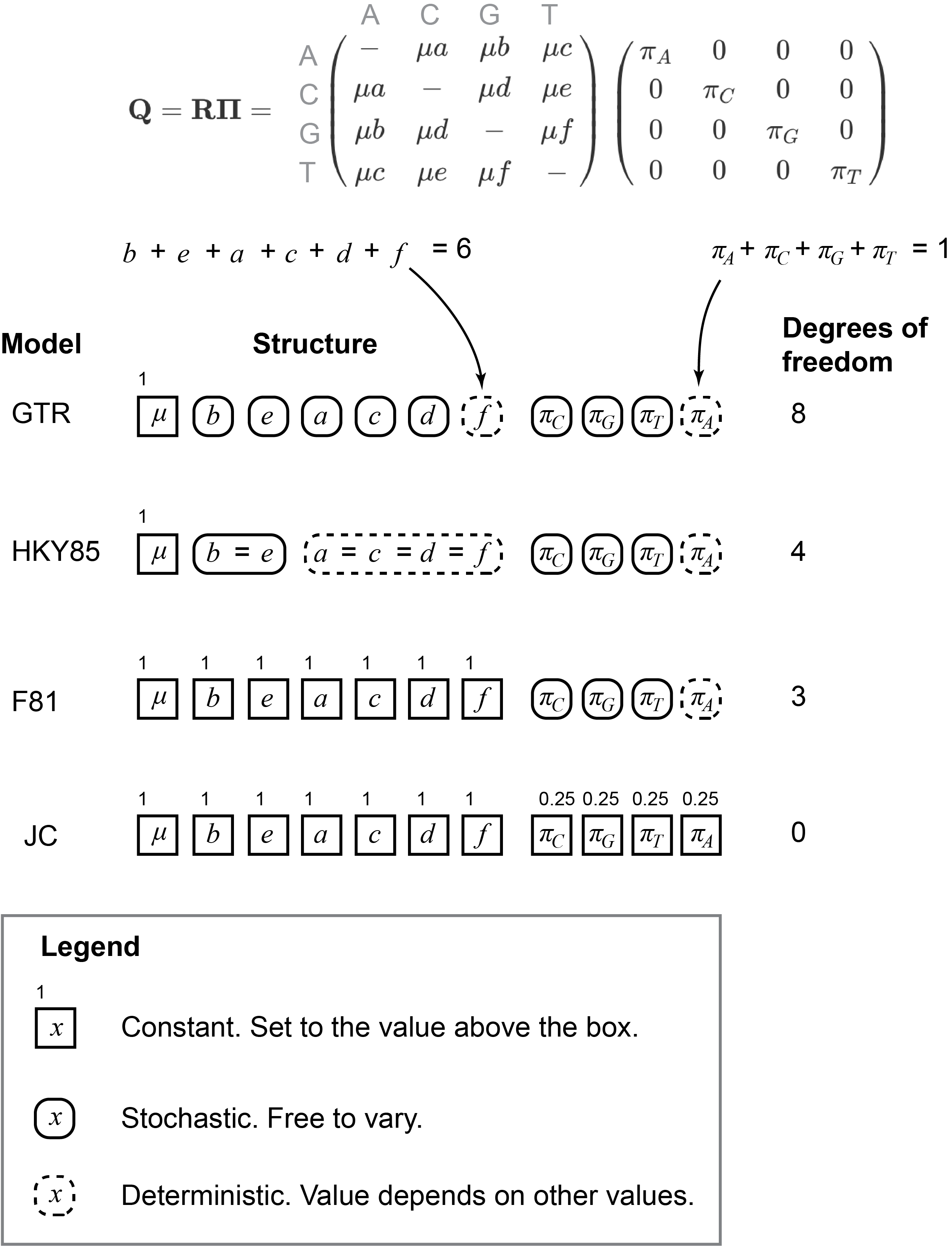
Figure 6.1: A hierarchical view of DNA substitution models. The number of degrees of freedom is determined by the number of independent stochastic parameters (boxes with rounded corners). All other parameters are either constant (set to a specific value ahead of the analysis; boxes with straight lines) or deterministic (their value depends on the value of other parameters according to specified relationships; boxes with dashed lines). Here \(\mu=1\), such that the branch lengths in the phylogeny are the expected amount of evolutionary change. The models are listed from top to bottom by increasing nestedness. Rates are ordered so that transitions and transversions are adjacent. Any model could be realized as a subset of the possible parameter space of the models above it. The visual nomenclature is inspired by Hohna et al. (2014).
The number of stochastic parameters in a model is referred to as the degrees of freedom, \(df\). You can think of it is the number of knobs that can be turned freely during the analysis. Models that have higher degrees of freedom are often referred to as more complex than models with fewer degrees of freedom.
The GTR model has \(df=8\). There are \(5\) stochastic relative rate parameters and \(3\) stochastic equilibrium frequencies (Figure 6.1). The other models we have seen are nested within this. By nested I mean that they can take on a smaller subset of the parameter values than the more complex model can. Models that are nested within other models have a smaller degree of freedom. See the iqtree DNA model documentation for a longer list of models.
The HKY85 model has \(df=4\) (Figure 6.1). There is \(1\) stochastic relative rate parameter, which determines the transition to transversion ratio. There are the same \(3\) stochastic equilibrium frequency parameters as in the GTR model. There are many values that a GTR model can take that an HKY85 model cannot, for example \(b\) can differ from \(e\) in GTR but not in HKY85. Every value that HKY85 can take can also be taken by GTR. For example, in HKY85 \(b=e\), and in GTR \(b\) and \(e\) are independent stochastic variables that can be different or that can take on the same value. Because every possible value of HKY85 is also possible in GTR, and GTR has more degrees of freedom than HKY85, HKY85 is nested within GTR.
Likewise, F81 is nested within HKY85 (and therefore GTR as well). It has \(df=3\), the same \(3\) stochastic equilibrium frequency parameters as in the GTR and HKY85 models. All the relative rates are constant and set to \(1\). Any value that F81 can take can also be taken by HKY85 or GTR.
The first model we introduced, JC, has \(df=0\). All the relative rates are constant at \(1\), and all the equilibrium frequencies are constant at \(0.25\). In typical use, \(\mu=1\). All the other models mentioned above have stochastic parameters that can take on these values, so JC is nested within them all.
Though nested models always have different degrees of freedom, there is no guarantee that models with different degrees of freedom have a nested relationship. It could be that the simpler model has some stochastic parameters that are not stochastic in the more complex model, even though the more complex model has a greater number of free parameters overall. That would allow the simpler model to take on values that the more complex model cannot, violating the nested relationship. When evaluating nestedness it is therefore critical to consider model structure, not just the degrees of freedom.
6.1.2 Evaluating models
In our previous examinations of inference, we used likelihood as an optimality criterion when looking for the phylogeny that best explains our data. Similarly, we can search for the model that best explains the data. We can pick a reasonable phylogeny and evaluate the likelihood of the data under each of the models we would like to consider. In each case we also optimize the model parameter values for each model to make sure we are comparing the models in the best possible light.
We can then make a series of pairwise comparisons between models, where we consider the ratio of their likelihoods. This is the gist of a likelihood Ratio Test (LRT). Instead of considering the ratio of likelihoods, we can consider the difference in their log likelihoods since:
\[\begin{equation} \Delta = ln(\frac{a}{b}) = ln(a) - ln(b) \tag{6.1} \end{equation}\]
If this difference \(\Delta\) is positive, then the model corresponding to \(a\) is more likely. If it is negative, then the model corresponding to \(b\) is more likely.
Let’s say we are comparing GTR to HKY85, and we denote the likelihood under GTR as \(L_{GTR}\) and the likelihood under HKY85 as \(L_{HKY85}\). We’ll put the model with more parameters, GTR in this case, in the numerator, i.e., set \(a\) above to \(L_{GTR}\) and \(b\) to \(L_{HKY85}\).
\[\begin{equation} \Delta = ln(\frac{L_{GTR}}{L_{HKY85}}) = ln(L_{GTR}) - ln(L_{HKY85}) \tag{6.2} \end{equation}\]
One way to proceed would then be to select GTR if \(\Delta>0\), and HKY85 if \(\Delta<0\). This wouldn’t be a good way to go, though, since it would pick GTR every single time. The reason is that HKY85 is nested within GTR. That means that the best possible likelihood under HKY85 is also available under GTR. Because it has more degrees of freedom, GTR has many other possible values, and chances are very good that one of those will be more likely than the parameter values that were most likely under HKY85. If comparing two nested models, the model with more degrees of freedom will never have a likelihood lower than the simpler model.
This would seem to imply that more complex models are always better, but they are not. As we add degrees of freedom, we are adding stochastic parameters that must be estimated from the data. In a very extreme case, we clearly couldn’t estimate an infinite number of parameters from a finite dataset – there wouldn’t be enough information to independently assess each parameter. But there are challenges even with a relatively small number of parameters. If we add too many model parameters, we can over-fit. Essentially, if there are too many model parameters we can make any phylogeny look good by adjusting the model parameters. This makes it more difficult to optimize the topology and branch lengths based on their impact on the likelihood. The data have finite information, and the more information we use to estimate model parameters the less we have to estimate the phylogeny.
When comparing nested models, the question therefore isn’t whether one model has higher likelihood than the other, but whether the increase in likelihood one gets from adding parameters is worth the cost of adding the parameters. There are a few different ways to make this cost/benefit analysis.
The simplest is to slightly modify the way we compare the log likelihoods, so that their difference is distributed according to a \(\chi^2\) distribution with degrees of freedom equal to the difference in degrees of freedom of the models:
\[\begin{equation} \delta = 2(ln(L_{1}) - ln(L_{0})) \tag{6.3} \end{equation}\]
We can compare this test statistic \(\delta\) to the appropriate \(\chi^2\) distribution to assess if the more complex model has a significantly greater likelihood. If not, we stick with the simpler model. It is important to note that it is only appropriate for comparing nested models.
There are a few challenges to applying the LRT to model selection in phylogenetics (Posada and Buckley 2004). One issue is that the test presumes that one of the models is correct (Zhang 1999), but in phylogenetics models are always simplifications of the evolutionary process at hand. The impact of violating this assumption varies across data sets and analyses, but can lead do undesirable behavior in real-world applications.
There are two other approaches commonly used in phylogenetic model selection. Where \(L_i\) is the likelihood under model \(i\), \(k_i\) is the degrees of freedom for the model, and \(n\) is sample size (e.g., number of sites in the alignment), these are the Akaike Information Criterion (AIC):
\[\begin{equation} AIC_i = 2k_i - 2ln(L_i) \tag{6.4} \end{equation}\]
And the Bayesian Information Criterion (BIC):
\[\begin{equation} BIC_i = k_iln(n) - 2ln(L_i) \tag{6.5} \end{equation}\]
To apply either of these criteria, they are calculated for each model and the model with the lowest value is selected. Adding parameters increases the value, penalizing any increase in likelihood they provide. These criteria have multiple advantages over LRT, including that they can be used to compare non-nested models (Burnham and Anderson 2002).
To decide whether to use LRT, AIC, or BIC model selection criteria, you need to run a model selection criterion selection analysis. Just kidding. To decide which to use, you should apply your knowledge of phylogenetic methods critically. In many cases, these different approaches will lead to very similar decisions about model selection. As an example of a fairly typical approach, the program iqtree runs AIC and BIC analyses, but proceeds under the model selected by BIC unless you explicitly step in to apply a different model. If, on inspection of the analysis results, you find that AIC selects a very different model, it would be prudent to run your analyses under that model as well to see if it leads to differences that are relevant to the questions that motivate your project.
6.1.3 Adding complexity to DNA evolution models
The GTR model, and its nested derivatives, capture only a small subset of evolutionary processes and therefore can’t describe many of patterns in observed data. One of the most obvious patterns you will notice when inspecting multiple sequence alignments is that the amount of variation is very different across sites. Some columns will be highly variable, while others are nearly constant. This pattern is due to extensive heterogeneity across sites in rate of evolution.
Two additional model features are often added to address this rate heterogeneity - I and G. These add additional degrees of freedom. The I parameter is the fraction of sites that are invariant and effectively have a rate of zero. G accommodates rate heterogeneity across sites that do vary (Yang 1994). This is modeled with a continuous \(\Gamma\) distribution that is divided into discrete rate categories, usually 4, to speed up computations. Sites are assigned to these different rate categories. To specify the shape of the \(\Gamma\) distribution, and therefore the rates of the categories, a parameter referred to as \(\alpha\) is used.
I and G can be added to GTR and its derivative models. Model selection routines usually examine a panel of models without these rate heterogeneity features, then with I, G, and I+G. The models with I+G are often selected, reflecting the importance of accommodating rate heterogeneity in real data.
6.2 Topological evaluation
Maximum likelihood inference gives a point estimate of the phylogeny – a single phylogeny (topology and branch lengths) that maximizes the probability of the observed data under the model. A maximum likelihood analysis will always return a single phylogeny, regardless of how strong the support for that phylogeny is or how much higher its likelihood is than that of other phylogenies. Presenting a phylogeny without any indication of topological support is akin to presenting an estimate of mass made from multiple observations without showing error bars. It is difficult to interpret the point estimate without having a sense of how much uncertainty there is.
6.2.1 Summarizing topological support
Before we get into how to assess support for a phylogenetic hypothesis, it is helpful to think about what that support means and how it is viewed on a phylogeny. Given a specific topology, such as a maximum likelihood phylogeny, how can we summarize and present support for that topology? I’ll refer to the topology we are evaluating as the focal topology.
Most methods that evaluate topologies generate a large set of phylogenies, which I’ll call the sample. Assessing support for a feature of the focal topology is a matter of assessing the frequency of phylogenies in the sample that also have that feature. We could assess the support for the focal tree as a whole by asking how frequent identical topologies are in the sample. But support can often be strong in one part of a phylogeny and weak in another. Reporting equivalence of the entire topology provides no window into that variation. This approach would also break down as taxa are added, which quickly increases the number of possible topologies and reduces the chances of any two analyses returning the exact same topologies, given the variation that is inherent in heuristic searches.
Branch frequencies are far more useful. It is helpful to think of a branch as a split (also sometimes called a bipartition) that separates all the taxa in a phylogeny into two groups - those on one side of the branch, and those on the other (Figure 6.2). We will consider two branches to be equivalent if they lead to the same taxon split. This allows us to discuss the equivalence of branches deep in a phylogeny, even when there are many other topological variations elsewhere in the phylogeny.
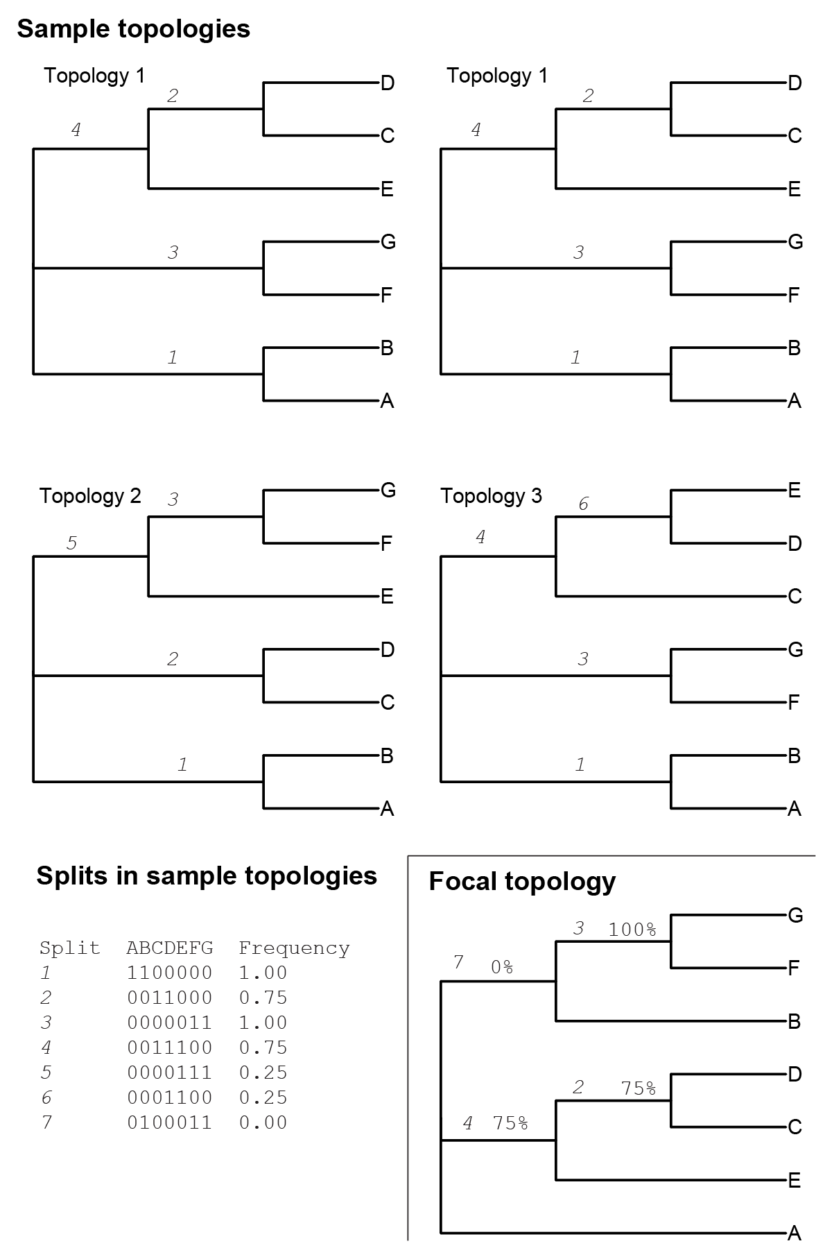
Figure 6.2: Four phylogenies in a sample, one focal phylogeny, and a table of splits found in all of these topologies. A split is a branch, identified by which taxa are split from each other by the branch. The splits table shows the binary encoding of each split, where taxa on the same side of the split have the same binary number (0 or 1). The assignment of 1 or 0 to a particular side of the split is arbitrary. Identical splits are labeled consistently above the branches throughout the figure. The frequency of the split is based on the proportion of sample phylogenies that contain the splits. The frequencies of the sample splits are shown as percentages on the branches in the focal topology.
We can consider each branch in the focal phylogeny independently. For a given focal branch, we count the fraction of phylogenies in the sample that have the same branch, as determined by producing an identical split in taxa. We consider this frequency as the support for the focal branch. If the frequency is 1, the branch was in all the phylogenies in the sample. If it is zero, it wasn’t present in any of the phylogenies in the sample. The interpretation of these frequencies, which are often reported as percents, depends on the method that was used to generate the sample.
It should be noted that these support values are often referred to as “nodal support values”, and are often drawn onto nodes. This is unfortunate, as they are branch support values. They are just commonly associated with child node of the branch rather than the branch itself. This obscures their meaning, and leads to serious problems when trees are re-rooted (Czech et al. 2017).
6.2.2 Bootstrapping
The most widely used approach to assessing confidence in maximum likelihood phylogenetic inference is the bootstrap (Felsenstein 1985). Given a data matrix where rows are taxa and columns are characters (nucleotide sites in the case of DNA) with \(n\) columns, bootstrapping generates a new matrix, also with \(n\) columns, by resampling from the the original matrix with replacement. Some columns from the original matrix won’t be sampled at all, some will be sampled once, and some will be sampled multiple times.
Bootstrapping is used to generate many new matrices (typically at least a hundred, but ideally 1000 or more), and maximum likelihood searches are then run on each matrix. This generates a sample of phylogenies. These can be examined in a variety of ways, but the most common is to evaluate the frequency of each branch of the maximum likelihood tree (generated form the original data matrix) in the sample of bootstrap phylogenies. A branch frequency of 100% indicates that a branch is always in the bootstrap replicates and is taken to be strong support. Support below 90% is generally considered weak.
Note that I am not using the term “significance” when referring to bootstrap support. This is because bootstraps don’t have a clear statistical interpretation. It is a scale that varies from \(0\) to \(1\), but is not itself a significance. It just indicates how frequently a branch is recovered when the data columns are resampled. This gives a sense of how broad support is for the branch across characters, but is quite complicated in reality. For example, some variation across bootstrap replicates is due to resampling, but sometimes it is just due to the stochastic nature of heuristic maximum likelihood searches.
Many phylogenetic inference programs do not run full independent maximum likelihood searches on each bootstrap replicate. Instead, they borrow information across replicates, such as optimal starting trees, to speed up the process.
6.3 Topology tests
Rather than assess the support of a particular focal topology, sometimes you want to assess how significant the difference in support is for specific phylogenies. There are several different topology tests that address these questions. They include the SOWH test (Swofford et al. 1996), KH test (Kishino and Hasegawa 1989), SH test (Shimodaira and Hasegawa 1999), AU test (Shimodaira 2002). Some of these are implemented in popular maximum likelihood software tools including iqtree (Minh et al. 2020). Their performance differs across conditions and their assumptions differ, so care should be taken in selecting and evaluating these tests (Goldman et al. 2000; Markowski and Susko 2023).