Chapter 3 Simulation

Here we will build the machinery to implement models of DNA evolution. Our first application of these models will be to simulate data.

3.1 Models

Models are representations of processes. They are abstractions in the sense that they leave out things that aren’t thought to be important, and they are idealized in the sense that they are deliberately simplified (Godfrey-Smith 2013, 21).

For some applications, it doesn’t matter if model structure reflects actual underlying processes, as long as it generates useful output (Breiman et al. 2001). For example, if data scientists at a large retail chain are trying to predict how much toothpaste they need to stock at each store, they likely don’t care if their models properly consider purchasing rates and all the other things that impact stock, so long as the the model does a reasonable job of making useful predictions. In science, though, we often care very much about the model because many of our questions have to do with the mechanisms that underlay the processes we are modeling. We don’t just want models that give us the right answer, we often want models that give us the right answer for the right reasons.

Statisticians often note that “All models are wrong but some are useful”, a common aphorism expanded from a quote by Box (1976). The goal of a model isn’t to be “right” in the sense of being a perfect explanation of data. Real data are far too complex for any model to do this. Instead, the most useful models strike a trade-off between simplicity and adequacy. They are as simple as possible, while adequately describing the phenomenon of interest. Adequacy is often in the eye of the beholder – one scientist will be perfectly happy with a model that makes reasonable rough approximations of a system, another scientist may be interested in second and third order effects for which more complexity is needed for adequate explanation.

Cartography is an interesting analogy for the way we will use statistical models. A “perfect” map would basically be a copy of the whole world, which wouldn’t be that much more useful than the world itself already is for many of the things you would like to do with a map. So all maps are simplifications (Figure 3.1). The simplification is often what makes the map useful.

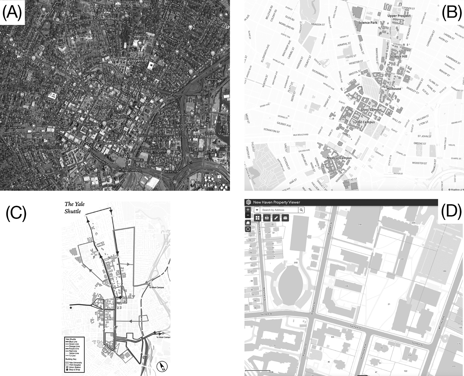
Figure 3.1: Four maps of the Yale campus, varying in complexity and focus. (A) A satellite image of New Haven, including much of Yale campus, from Google Maps. This image has a very large amount of information. (B) A street map of the same region, also from Google Maps. It has less information, but is more useful for some tasks such as navigation. (C) An even more simplified map, focused on showing the Yale Shuttle routes. (D) The New Haven property map of the region around Osborn Memorial Laboratory, showing property lines and plot numbers. Like (C) it is simple, but reflects different decisions about which information to discard or retain. This figure is inspired by the London maps that David Swofford uses in his own talks to make the same points.

Let’s examine one of the most common models, the linear model:

\[\begin{equation} y = mx+b \tag{3.1} \end{equation}\]

Here, \(y\) and \(x\) are variables. The model posits a linear relationship between \(x\) and \(y\). If you plot their correspondence in a plane you will get a line. \(m\) and \(b\) are model parameters. \(m\) is the slope of the line. It captures how much change there is in \(y\) for each unit of change in \(x\). \(b\) is the intercept. It is the value of \(y\) when \(x=0\).

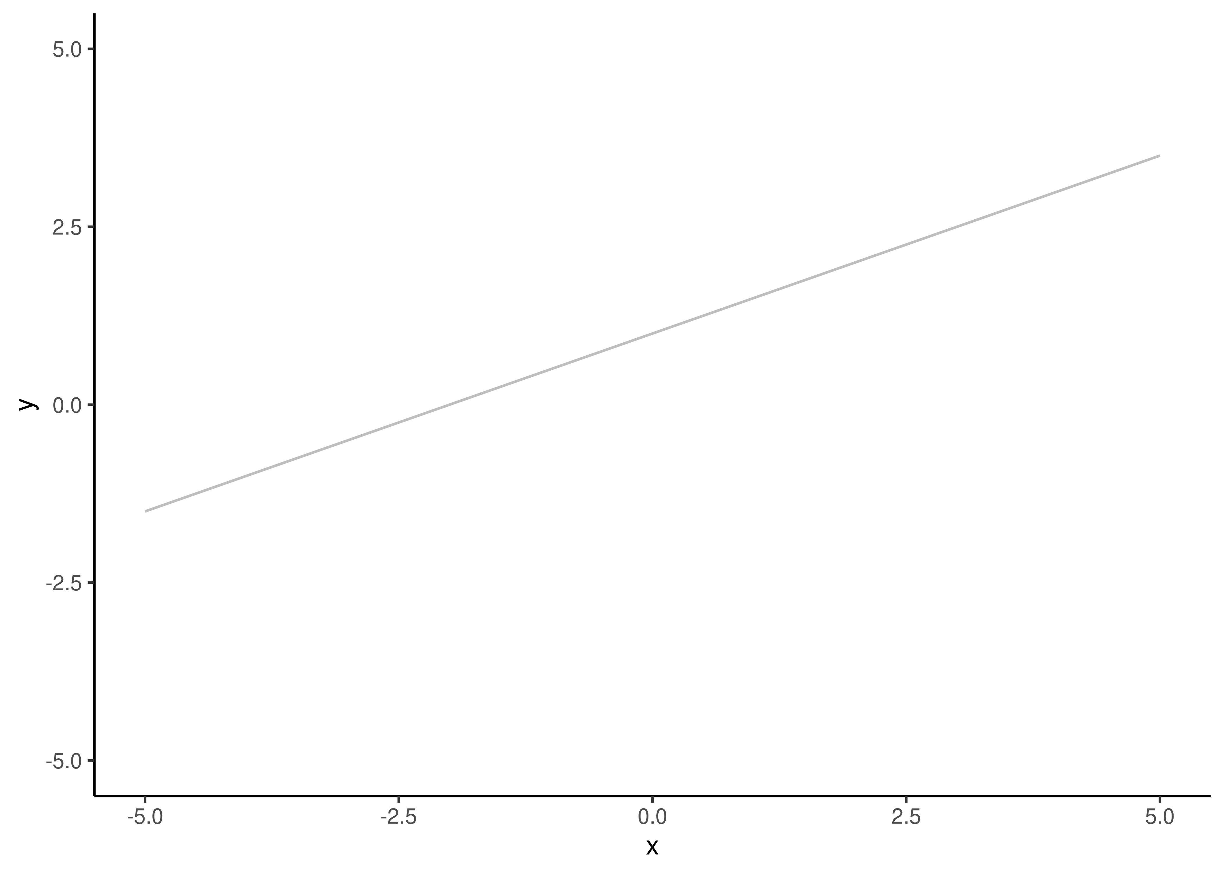
Figure 3.2: A linear model with \(m=0.5\) and \(b=1\).

There are a variety of useful things we could do based on these relationships between the model, model parameters, and values. Let’s consider \(x\) to be a variable that tell us something about the past and \(y\) to be a variable that tells us something about the present or future. Use cases then include:

• If we clamp the model (linear) and model parameters (specific values of \(m\) and \(b\)) according to prior knowledge, and clamp \(y\) according to observed data, we can estimate \(x\). In this case the model is like a time machine that allows us to look into the past.

• If we clamp the model (linear) and variables (\(x\) and \(y\)) according to prior knowledge, we can estimate model parameters \(m\) and \(b\). In this case the model is like an instrument that allows us to peer inside processes based on their inputs and outputs.

• If we clamp the model (linear) and model parameters (specific values of \(m\) and \(b\)) according to prior knowledge, and clamp \(x\) according to observed data, we can estimate \(y\). In this case the model is like an oracle that predicts the future.

• If we clamp the model (linear) and model parameters (specific values of \(m\) and \(b\)) according to prior knowledge, and clamp \(x\) according to values we make up, we can simulate \(y\). In this case the model is like a world-builder that tells us what we would expect to see under the specified conditions. This is very helpful for getting a sense of whether our models are working well (Do they generate results that look like what we see?), examining counterfactual situations that don’t exist, or building datasets to test software tools.

There are some deep connections here. For example, predicting the future is basically just simulating the future based on our model and what we already know about the past and present.

The models that we will use in phylogenetic biology tend to be more complex than the linear mode, but this general perspective of clamping and estimating different things still holds.

3.2 A simple model of evolution

Let’s start with a simple model of DNA evolution. At first we will also consider only a single nucleotide position along a single branch in a phylogeny (Figure 3.3). The goal is to build an intuitive integrated understanding of the mathematical and statistical relationships among:

• Model structure
• Model parameters
• Branch length
• State at the start of the branch (the nucleotide at the parent node)
• State at the end of the branch (the nucleotide at the child node)

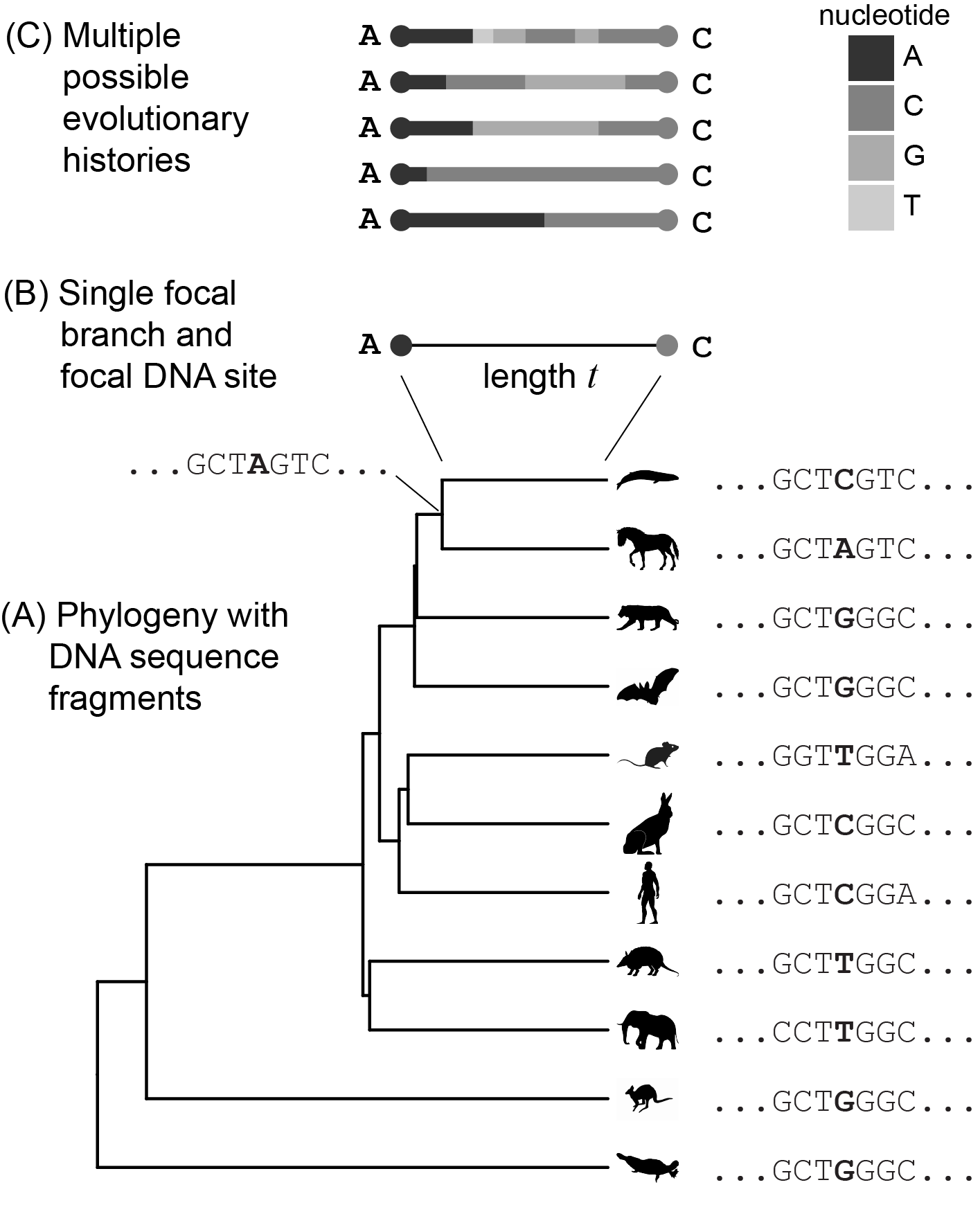
Figure 3.3: Our current goal is to model the evolution of a single site in a DNA sequence along a single branch in a phylogeny. (A) An example phylogeny, with DNA sequence fragments shown at the tips and one internal node. The site under examination is in color, and the branch under examination (at the top) is thicker than the rest. (B) A closeup of the focal branch, and the state of the focal site at its ends (the parent and child nodes). (C) Multiple mutational histories that are consistent with the starting and end states shown in (B), i.e. a cange from A to C.

Imagine that when the DNA is being replicated, most of the time the appropriate nucleotide is incorporated. Some fraction of the time, at rate \(\mu\), an event occurs where the appropriate nucleotides is replaced with a random nucleotide instead. In our model, the probability of selecting any of the nucleotides during one of these random replacement events is uniform (picking a C is just as probable as picking a G, for example), and the new nucleotide doesn’t depend in any way on what nucleotide was there before. It is as if you had a bag containing a large number of C, G, T, and A nucleotides at equal frequencies. As you built the new DNA strand, every so often you would replace the nucleotide you should be adding with one you instead select by reaching into the bag and picking at random.

Not all replacement events will result in an apparent change. Sometimes the appropriate nucleotide is selected by chance, even though it was picked at random. If, for example, the appropriate nucleotide was an A, under this model \(1/4\) of the time a replacement event occurs, an A is selected by chance and there is no apparent change. In such a case, there has not been a substitution, just a replacement in kind. If the A is replaced with any of the other three nucleotides we say there has been a substitution. Because three of the four possible outcomes of a replacement event result in a substitution, the substitution rate is \((3/4) \mu\). Because some events result in no apparent change, substitutions are only a subset of events and the substitution rate is lower than the replacement rate.

It might seem a bit odd to consider replacement events that don’t result in substitutions, but this follows naturally from a central feature we specified for the the model - the new nucleotide doesn’t depend in any way on what nucleotide was there before. If we had a process where replacements always resulted in substitutions, then excluding the replacement-in-kind events would require knowing which nucleotide should be placed so that we don’t select it.

3.2.1 Expected amount of change

For the simple process described here, there are two things to consider if we want to know the amount of evolutionary change. The first is the rate \(\mu\), and the second is the time over which the evolutionary process acts. In our example here, that time is the length of the branch under consideration in the phylogeny.

In Figure 3.4 each horizontal bar is a simulation over the same time interval (0-100 time units). Each black line on the bar is a replacement event randomly introduced by the computer according to our model. We use a different value of \(\mu\) for each simulation (as indicated on the vertical axis). In the bottom bar, where \(\mu=0\), there are no replacements (black bars) and therefore no substitutions (the whole bar is the same color). There are more replacement events as \(\mu\) increases along the vertical axis.

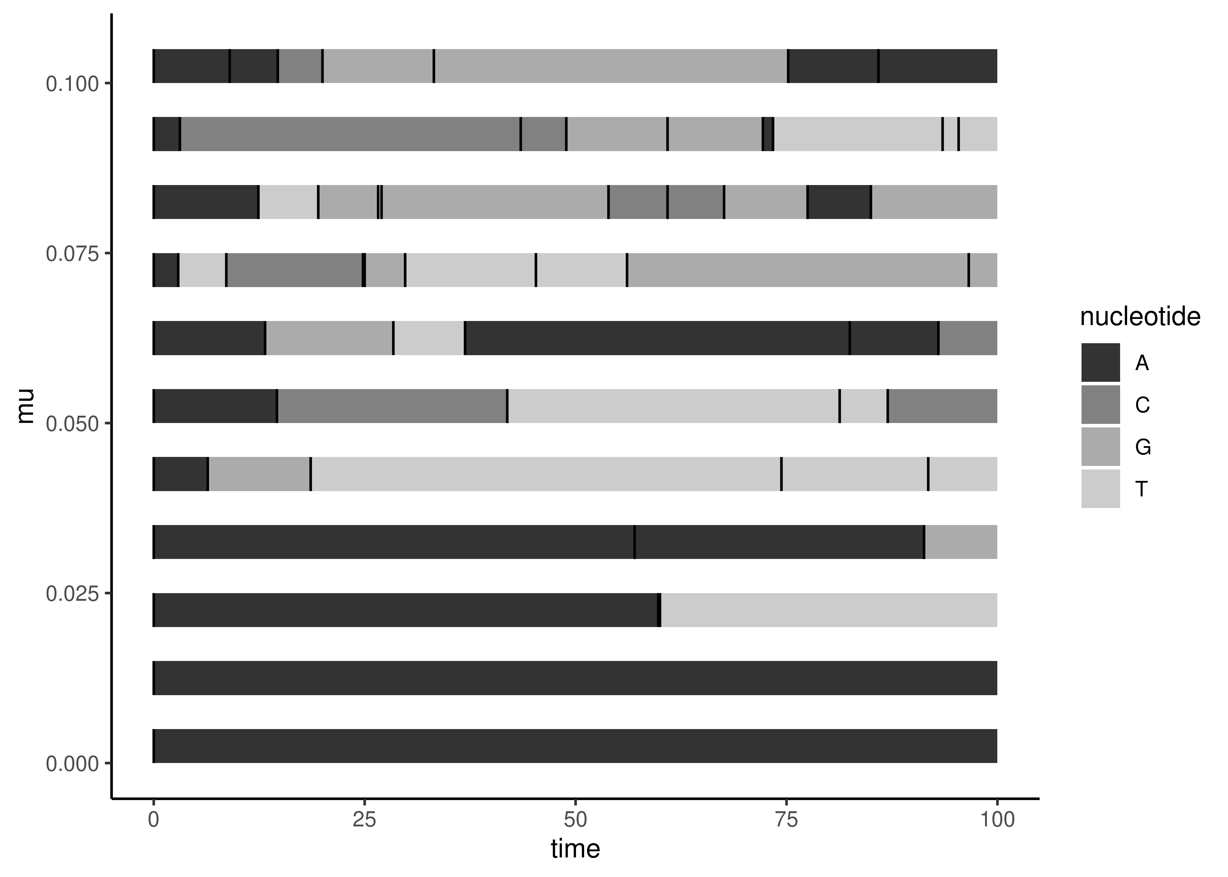
Figure 3.4: Each horizontal bar is a simulation of evolution of a single nucleotide position through time, \(t\), for a specified value of \(\mu\). Each simulation starts out as an A. Black vertical lines correspond to replacement events, which don’t all lead to substitutions (a new color).

As \(\mu\) increases (going up on the vertical axis), the number of replacement events over the same time interval increases (Figure 3.5). This reflects the simple linear relationship \(n=\mu t\), where \(n\) is the number of expected replacement events.

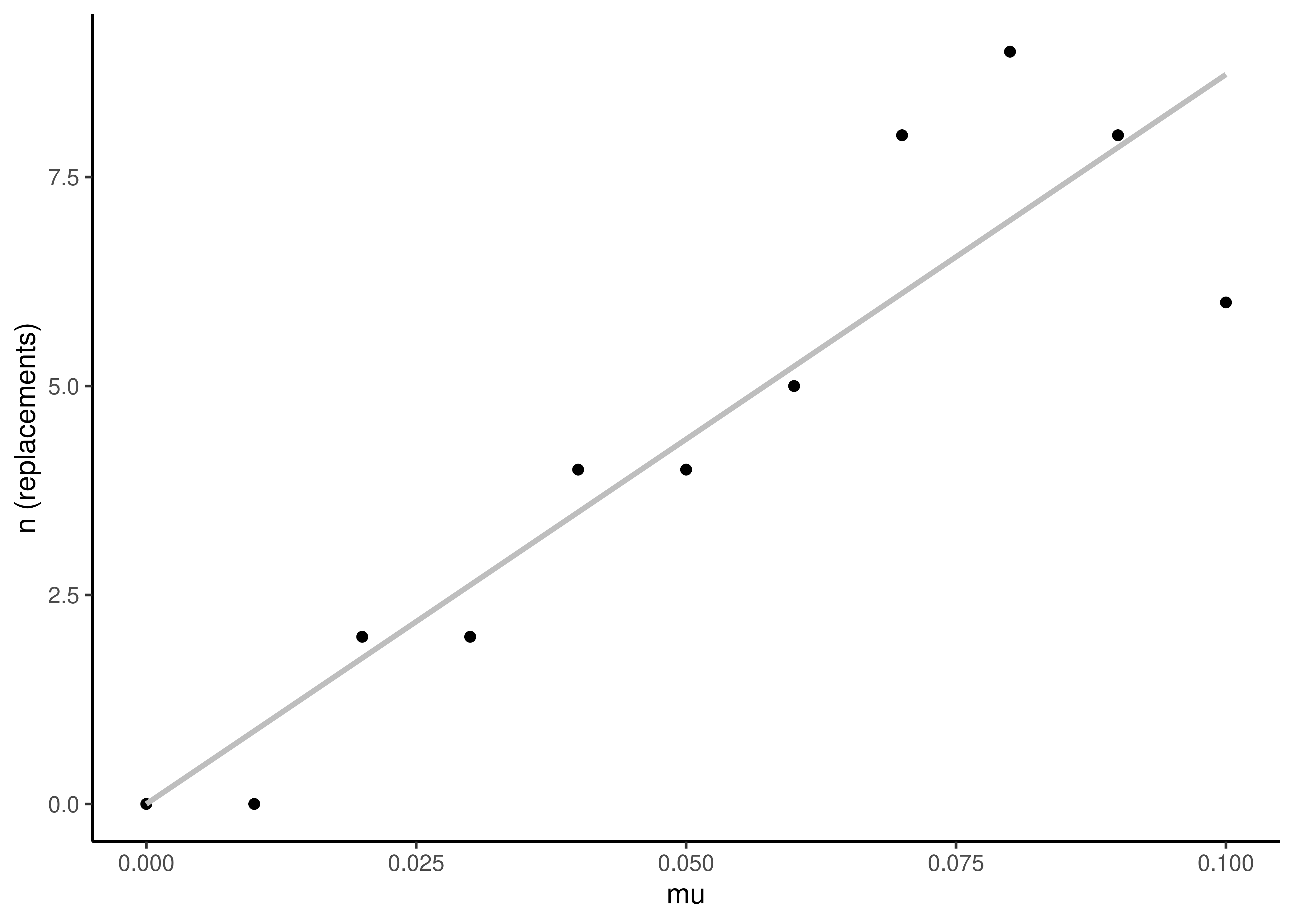
Figure 3.5: The number of replacement events increases linearly with the replacement rate \(\mu\). This plot is from the same simulation as that shown in Figure 3.4. The line is a linear model fit to the data. Since \(n=\mu t\), and in this case \(t=100\), the slope of \(n\) on \(t\) is estimated to be near 100.

Because of the linear relationship between the number of replacements and the product \(\mu t\), rate (\(\mu\)) and time (\(t\)) are conflated. In many scenarios you can’t estimate them independently. If there are a small number of replacements, for example, you can’t tell if there is a low rate over a long time interval, or a high rate over a short interval. Both would give the same resulting number of changes \(n\). Because rate (\(\mu\)) and time (\(t\)) are so often confounded in phylogenetic questions, often the rate is essentially fixed at one and the unit of time for branch lengths is given as the number of expected evolutionary change rather than absolute time (years, months, etc). You will often see this length as the scale bar of published phylogenies (Figure 3.6). The exception is when you have external information, such as dated fossils, that allow you to independently estimate rates and branch lengths in terms of actual time. Sometimes deconfounding \(\mu t\) isn’t important to the primary question of the investigator, sometimes it would be nice to know but can’t be done, and other times (such as in papers that date trees) it is the central question.

Figure 3.6: A published phylogeny (Zapata et al. 2015) with a scale bar indicating branch length in terms of the expected amount of evolutionary change, rather than absolute time.

3.2.2 Expected end state

The machinery above shows how a model can clarify the way we think about the expected amount of change along a branch. Many times, though, we want to know what the probability of a given end state is given a starting state, a model, and the amount of time elapsed. One way to anchor such a question is to think about the extremes - what do we expect after a very small amount of change (either a short time or a slow rate of change, or both), and what do we expect after a large amount of change?

The situation is most clear after a small amount of change (when \(\mu t\) is small) - we expect the end state to be the same as the starting state. If we start with an A, for example, if there is very little change we expect to end with an A (Figure 3.7, left side). In this situation, the starting state tells us a lot about the end state. Not much else matters.

What should we expect, though, if there has been a large amount of change (when \(\mu t\) is large)? Can we know anything at all? It turns out that we can. If there have been many replacements, one after the other, than the initial starting state doesn’t matter because whatever was there initially will probably have been replaced multiple times. It is as if had been erased and written over. If the starting state doesn’t contain information about the end state, what does?

Since replacements are coming from the bag that you are picking the nucleotides at random from, that bag has information about the expected states after a large number of changes. Given enough evolutionary time, our simple model will lead the expected frequency of each nucleotide in the evolving sequence to be the same as their frequencies in the bag. Since we specified that you have the same chance of grabbing any nucleotide from the bag, eventually the probability of having each of the our nucleotides is the same, 25% (Figure 3.7, right side). If you started with a sequence that had an A and let it evolve 100 times, after enough evolutionary time had passed to reach equilibrium you would expect to get 25 C’s, 25 G’s, 25 T’s, and 25 A’s.

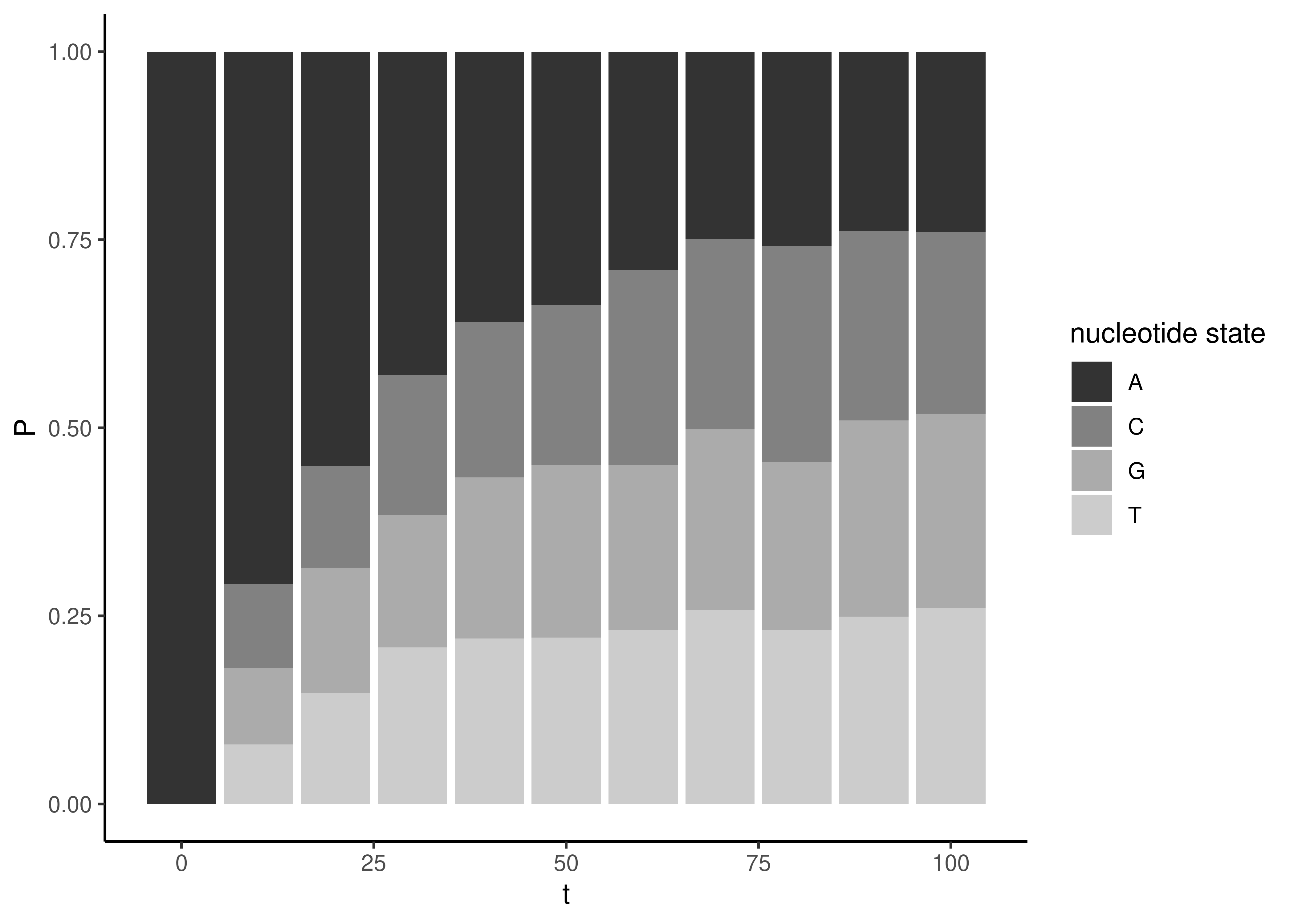
Figure 3.7: Stacked bar plots indicating the frequency of each nucleotide after simulated evolution for a specified amount of time. The rate of evolution is \(\mu=0.050\). There are 1000 replicate simulations for each value of time. At time \(t=0\) (no evolution), the end result is always the same as the initial value, which is fixed at A in these simulations. As the length of time increases, the four nucleotides converge on equal proportions of 0.25 each.

3.2.3 Analytical approach

In all the examples above, I simulated replacement events by randomly generating them at the specified rate. To get the end state, I then just retained the last state. You could take this approach to assessing the probability of different outcomes in actual analyses, but it gets very computationally expensive. It would be better to have an equation to solve for the probabilities directly. That isn’t always possible for a model, but it is in this case.

The process of change that our simple model describes is similar to compound interest. We have something in hand, apply a process to it, then take the output and apply that same process again. Over and over. In the case of compound interest, that something is money and the process is growth. In the case of our model, the something is a DNA site and the process is mutation. In both cases, we take as inputs a starting state, a rate of change, and an amount of time, and as an output get the expected end state. To get the expected end state as a function of time elapsed, given a rate of change, we can use exponential functions. For example, here is the exponential function for calculating a balance at time \(B(t)\) given the initial balance \(B_0\) and an interest rate \(r\):

\[\begin{equation} B\left(t\right) = B_0 e^{r t} \tag{3.2} \end{equation}\]

For our sequence evolution model, we need two exponential functions (Swofford et al. 1996):

\[\begin{equation} P\left(t\right) = \frac{1}{4} + \frac{3}{4} e^{-\mu t} \tag{3.3} \end{equation}\]

\[\begin{equation} P\left(t\right) = \frac{1}{4} - \frac{1}{4} e^{-\mu t} \tag{3.4} \end{equation}\]

Equation (3.3) shows the probability of the final state being the same as the beginning state. So if you start with an A, this would give you the probability of remaining an A after time \(t\) given a specific value of \(\mu\). Equation (3.4) is the probability of each of the three end states that are different from the starting state. If you start as an A, this is the probability of changing to a G, for example. It is also the rate of C to T, G to A, etc…

Consider what happens to these equations in the extremes we considered above when examining Figure 3.7. If \(\mu\) or \(t\) are zero, we expect no change (Figure 3.8, left side). In that case we get \(e^0\), which is 1. Equation (3.3) becomes \(1/4 + 3/4\), which is 1. So there is a probability of 1 that, after no change, the end state is the same as the beginning state. Likewise, Equation (3.4) becomes \(1/4 - 1/4\), which is 0. So after no change the end states that differ from the beginning state each have probability 0.

Now consider the case after infinite change (or just a large amount of change, as in the right side of Figure 3.8). If \(\mu\) or \(t\) are infinity, then \(e^{-\mu t}\) becomes \(e^{-\infty}\), which is 0. In that case, Equation (3.3) becomes \(1/4 + 0\), which is simply \(1/4\). Likewise, Equation (3.4) becomes \(1/4 - 0\), which is also \(1/4\). So all the nucleotides (the one that you started with, and the three other states that substitution can lead to) all have the same equal frequency of \(1/4\). This reflects the fact that the frequency of drawing each of these from the bag was \(1/4\).

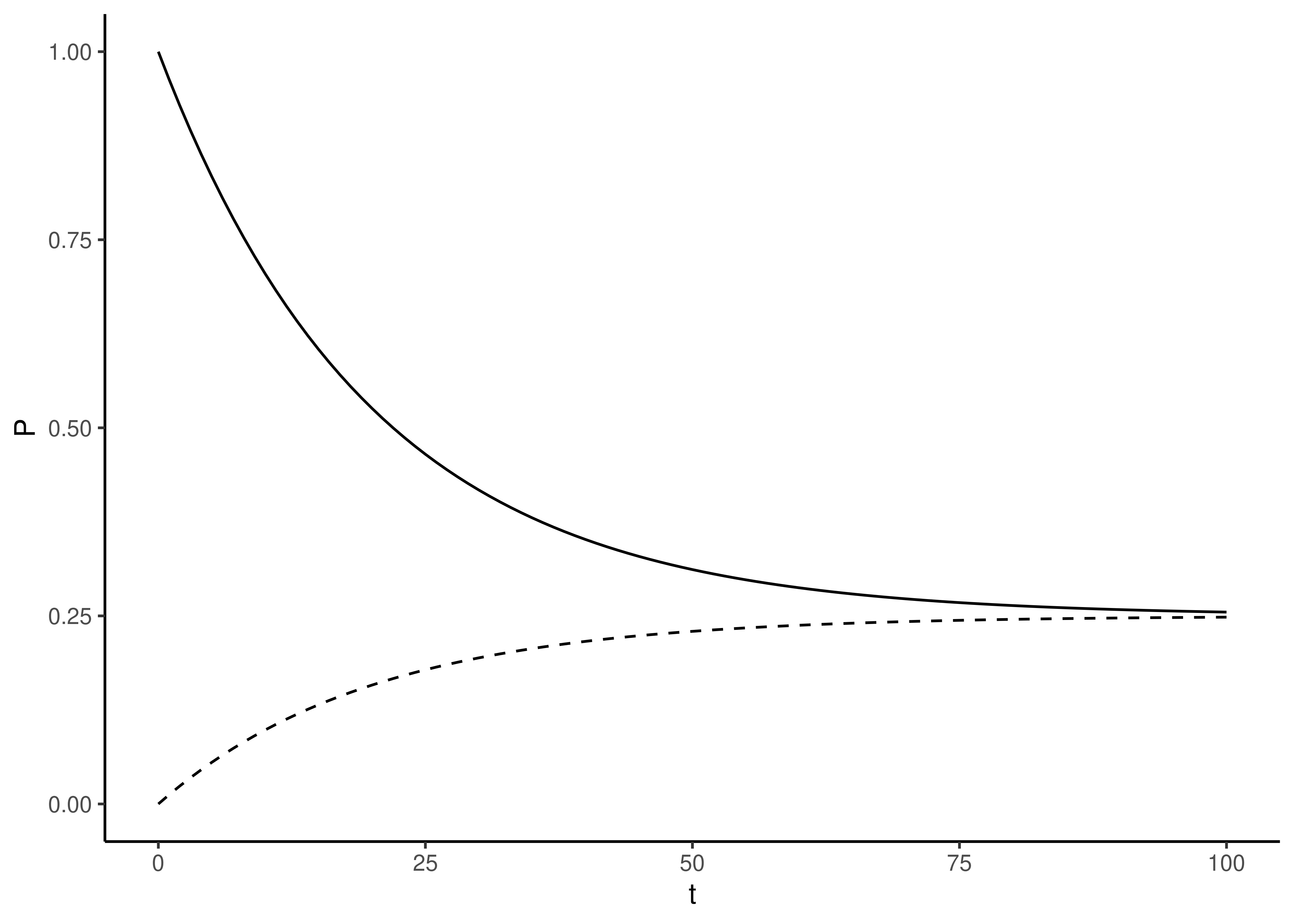
Figure 3.8: The probability of observing a particular end state at time \(t\), given the start state A and \(\mu=0.05\). The solid line is the probability of observing the original start state (as described by Equation (3.3)), the dashed line is the probability of observing each of the three other states (as described by Equation (3.4)).

We can reorganize things a bit (Figure 3.8) to get a plot like that of Figure 3.7, but derived from Equations (3.3) and (3.4) instead of from actual simulations of changes along branches.

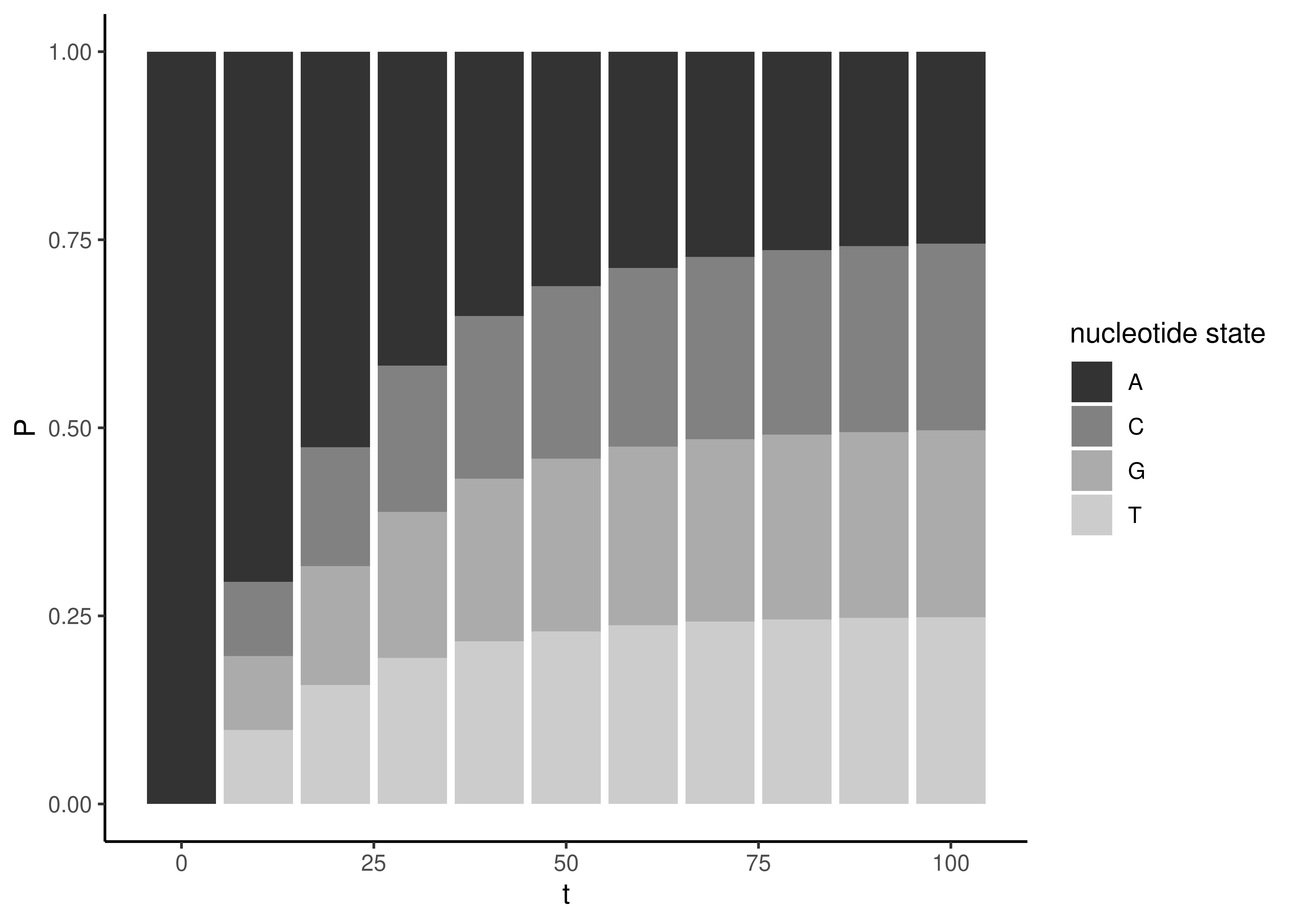
Figure 3.9: Stacked bar plots indicating the frequency of each nucleotide after evolution for a specified amount of time. The rate of evolution is \(\mu=0.050\). The starting state is set at A, so the probability of observing an A is described by Equation (3.3). The other three nucleotides, C, G, and T, are described by Equation (3.4). At time \(t=0\) (no evolution), the probability that the state is the same as at the start is 1.0. As the length of time increases, the four nucleotides converge on equal probability of 0.25 each.

Let’s put this back into a biological context. Our simple model allows us to calculate the probability \(P(t)\) of a given nucleotide state at the end (child node) of a branch given:

• The nucleotide state at the beginning (parent node) of the branch
• Replacement rate \(\mu\)
• Length of the branch \(t\)

This is powerful stuff. We could do a variety of things with this model machinery, for example:

• Simulate evolution along a branch by sampling nucleotides for the child node from this probability distribution
• Ask the probability of a given starting state given an end state
• Evaluate how reasonable our \(\mu\) model parameter value is. If, for example, we have a tree with very short branches that had different states at their parents and children, we might be skeptical of a low \(\mu\) value.

3.3 Generalizing the simple model

The model we built above only has one parameter that can vary, \(\mu\), so we can describe the model parameters very simply. This is convenient, but leaves some of the things that are happening under the hood a bit opaque. Let’s rewrite this simple model in a way that makes it a bit clearer how we are using this parameter, and also reveals some other parameters that are there but that we ignored until now because they were clamped. First, we need to represent the model as a \(4\times4\) rate matrix, which we will call \(\mathbf{Q}\), as defined in Equation (3.5). Each row corresponds to one of the four possible nucleotides (A, C, G, T, in that order from top to bottom), and each column corresponds to one of the four possible nucleotides (A, C, G, T, in that order from left to right). Each of the elements in the matrix is the instantaneous rate of change from the nucleotide of the corresponding row, to the nucleotide of the corresponding column.

\[\begin{equation} \mathbf{Q} = \left(\begin{array}{cccc} -3\mu\pi & \mu\pi & \mu\pi & \mu\pi\\ \mu\pi & -3\mu\pi & \mu\pi & \mu\pi\\ \mu\pi & \mu\pi & -3\mu\pi & \mu\pi\\ \mu\pi & \mu\pi & \mu\pi & -3\mu\pi\\ \end{array}\right) \tag{3.5} \end{equation}\]

Recall that \(\mu\) is the rate of any replacement event happening. That replacement event could be an A, C, G, or T. Only three of these replacements lead to a substitution, since replacing with the original nucleotides does not lead to a change. To find the rate of specific replacements happening, as we need to do for the elements of this matrix, we need to apportion the total replacement rate \(\mu\) to specific nucleotides. We can do that with a new term \(\pi\), which is the name we will give to the equilibrium frequency of each state. This corresponds to the frequency of each nucleotide in the bag we randomly sampled from. In our simple model, \(\pi=0.25\) for all nucleotides. Because \(\pi\) was clamped and wasn’t free to vary, it was essentially invisible in the way we previously described the model.

The off-diagonal elements of \(\mathbf{Q}\) give the rates of substitutions, and are all \(\mu \pi\). But what’s up with the diagonal elements? We pick these diagonal elements to be whatever value leads the rows to sum to 0. The basic intuition of this is that we aren’t creating or destroying nucleotides, just replacing them. So the net change needs to be 0. Since there are three substitutions in each row, and each substitution has rate \(\mu \pi\), these diagonal elements are set to \(-3 \mu \pi\). The negative rates for the diagonal elements can be thought of as a rate of leaving the current state, while the positive off diagonal rates correspond to entering new states.

There is a lot going in in \(\mathbf{Q}\). To make sense of it all, it helps to factor it out into two parts (Swofford et al. 1996). The first is a \(4\times4\) matrix \(\mathbf{R}\), which has all the rates, and the second is a \(4\times4\) matrix \(\boldsymbol{\Pi}\) that has the equilibrium frequencies on its diagonal and 0 everywhere else (Equation (3.6)).

\[\begin{equation} \mathbf{Q} = \mathbf{R}\boldsymbol{\Pi} = \left(\begin{array}{cccc} -3\mu & \mu & \mu & \mu\\ \mu & -3\mu & \mu & \mu\\ \mu & \mu & -3\mu & \mu\\ \mu & \mu & \mu & -3\mu\\ \end{array}\right) \left(\begin{array}{cccc} \pi & 0 & 0 & 0\\ 0 & \pi & 0 & 0\\ 0 & 0 & \pi & 0\\ 0 & 0 & 0 & \pi\\ \end{array}\right) \tag{3.6} \end{equation}\]

(This factoring is possible because of the way matrix multiplication works. For a refresher on matrix multiplication, this video explains how to do it operationally, and this series of videos explains what it is actually doing.)

\(\mathbf{Q}\) is the instantaneous rate matrix – it specifies the particular amount of change we expect over a short period of evolutionary time. But as we discussed before, we often want to know the probability of ending with a particular state if you start with a particular state and let it evolve along a branch of a given length. Before, when we were keeping things as simple as possible, we used the exponential Equations (3.3) and (3.4) for this. They took as input the overall replacement rate \(\mu\) and the length of the branch \(t\). Now we want a similar equation, but we want to provide the rate matrix \(Q\) rather than the single parameter \(\mu\). Again we can just use an exponential function, and it actually has a much simpler form.

\[\begin{equation} \mathbf{P}\left(t\right) = e^{\mathbf{Q} t} \tag{3.7} \end{equation}\]

Raising \(e\) to the power of a matrix like this is known as matrix exponentiation, and it returns a matrix with the same dimensions as the matrix in the exponent. This new matrix \(\mathbf{P}(t)\) is therefore also a \(4 \times 4\) matrix. As for \(\mathbf{Q}\) and \(\boldsymbol{\Pi}\), and \(\mathbf{R}\), each row corresponds to one of the four possible nucleotides (A, C, G, T), and each column corresponds to one of the four possible nucleotides (A, C, G, T). Each of the elements in the matrix is the probability of going from the nucleotide of the corresponding row to the nucleotide of the corresponding column over a branch of length \(t\). Given the single rate parameter and uniform equilibrium frequencies, the diagonal elements are each Equation (3.3), and the off diagonal elements are each Equation (3.4).

Wow! This was a lot of work to write a really simple model in a much more complicated way. Now we can start to reap the rewards of describing this simple model in this form.

3.4 Expanding the models

The mathematical, statistical, and computational machinery above describes the evolution of one DNA site along one branch in a phylogeny (Figure 3.3) according to a simple model. In fact, this is the simplest possible model of DNA evolution, named JC69 after the folks who described it in 1969 (Jukes and Cantor 1969). It is only one free parameter – the rate of evolution \(\mu\). It is highly idealized – there are many important facts about DNA and DNA evolution that we deliberately omit.

The simplicity of JC69 makes it a useful starting place to understand how models of DNA evolution work, but it is too simple to be very useful in practice. There are many other biological aspects of sequence evolution we might want to consider, including that:

• The nucleotides C, G, T, and A are often not found at an equal frequency of 0.25 each. Since the nucleotides form base pairs in organisms with double stranded genomes, C and G are found at the same frequency and T and A at the same frequency. Furthermore, the frequency of the four nucleotides must add to 100%. Therefore, the frequency of all four nucleotides can be summarized with a single number, usually given as the GC content – the percent of sites that are G or C. For example, the human genome has a GC content of 41%, which indicates nucleotide frequencies of 0.205 G, 0.205 C, 0.295 T and 0.295 A. This is quite different than the equal frequencies of 0.25 for all nucleotides expected by the JC69 model.

• The rates of mutation between different nucleotides is not the same. This is in part because some nucleotides are shaped more like others, and are more likely to be substituted for each other by mistake. In particular, A and G tend to be substituted for each other because they have two rings, and C and T tend to be substituted for each other because they have one ring. These changes between A/G and C/T are referred to as transitions. All other substitutions are called transversions, and are each less likely.

To accommodate each of these deviations from JC69, we need to add parameters to the model to explain the added complexity. There are all kinds of parameters we could add one by one, and in fact that is how the field proceeded in the decades after JC69 was described. Rather than build the models up in that way, though, it is actually easier to describe a general model that these other models, including JC69, are special cases of.

\[\begin{equation} \mathbf{Q} = \mathbf{R}\boldsymbol{\Pi} = \left(\begin{array}{cccc} - & \mu a & \mu b & \mu c\\ \mu a & - & \mu d & \mu e\\ \mu b & \mu d & - & \mu f\\ \mu c & \mu e & \mu f & -\\ \end{array}\right) \left(\begin{array}{cccc} \pi_A & 0 & 0 & 0 \\ 0 & \pi_C & 0 & 0 \\ 0 & 0 & \pi_G & 0 \\ 0 & 0 & 0 & \pi_T \\ \end{array}\right) \tag{3.8} \end{equation}\]

(To keep things compact, I have followed the convention of placing \(-\) in the diagonal elements, which is short for “whatever it takes to make the rows of \(\mathbf{Q}\) sum to 0”.)

This model (Equation (3.8)) is called the General Time Reversible (GTR) model of DNA sequence evolution. It is General because it has parameters that allow many things to vary independently. The \(\pi_A ... \pi_T\) parameters allow the equilibrium frequencies to differ for each nucleotide. The \(a ... f\) parameters adjust \(\mu\) so that rates can differ. For example, the instantaneous rate of change from A to C can be different from that of A to G by setting \(a\) and \(b\) to different values. It is Time Reversible because we don’t have different rate parameters for every single off-diagonal element, but instead mirror them. This means, for example, that the rates of change from A to C and from C to A are both the same, \(\mu a\). There are a few motivations for this. It keeps the total number of parameters down. It also reflects what is observed biologically. And it means that we don’t need to know the direction of time along a branch to calculate \(\mathbf{P}(t)\). This last point is very important since we often don’t know where the root of a tree is when we want to calculate these probabilities. It also turns out to be convenient and efficient for phylogenetic inference software tools to reroot phylogenies without changing these probabilities as they make calculations on phylogenies.

If we let all the parameters in the GTR model (Equation (3.8)) be free, it is quite complex. We would have to estimate them all from data. The alternative is to clamp some of them. In fact, by comparison of Equations (3.6)) and (3.8), we can see that JC69 is a clamped version of GTR where \(\pi_A=\pi_C=\pi_G=\pi_T=0.25\) and \(a=b=c=d=e=f=1\). Only \(\mu\) is left free in JC69.

There are a variety of other commonly used models that clamp these parameters in different ways, some leaving more freedom than others. Some that are widely used and have very specific biological motivation have their own names, like JC69 (the motivation for this model is that it is so simple). Examples of other named models include:

• HKY85 differs from GTR in setting some rate modifiers equal to each other so that there are two rates, \(b=e\) for transitions (A to G, and C to T) and \(a=c=d=f\) for transversions (all other changes). It still lets all the \(\pi\) parameters vary independently.

• F81 differs from HKY85 in that it sets all the rate modifiers to 1, so that \(a=b=c=d=e=f=1\). It is almost as simple as JC69, except that the \(\pi\) parameters vary independently.

We now have a more complex model of DNA evolution that we can simplify by setting the parameters to equal each other and/or clamping them to specific values. It can accommodate much of variation observed in actual DNA sequence data. We could use it to simulate data just as we did in Figure 3.7, but taking into consideration things like unequal nucleotide frequencies and differences in rates of change between nucleotides. This is getting us much closer to something that provides real biological insight.

3.5 Plugging some numbers into the expanded model

Now that we have a framework for specifying a model with unequal equilibrium frequencies and different rates of change between different nucleotide pairs, let’s build a specific case of a model and use it to simulate some data. That means we need to pick some actual model parameters, plug them into \(\mathbf{R}\) and \(\boldsymbol{\Pi}\) to get \(\mathbf{Q}\), and then exponentiate that to get \(\mathbf{P}(t)\). We can then use that to simulate changes in a single nucleotide along a branch. This will be a mathematically grounded version of the schematic in Figure 3.3B.

We are using a mammal tree, so let’s pick some parameter values that roughly approximate what we see in mammals. Rather than set all the parameters independently, let’s set up an HKY85 model, which accommodates non-uniform base frequencies and different transition/ tansversion ratios. First, we can clamp \(\mu=1\). This basically just means the branch lengths will be in units of expected evolutionary change. Transitions (captured by parameters \(b\) and \(e\)) are on the order of 4 times more frequent than transversions (captured by parameters \(a\), \(c\), \(d\), and \(f\)) in mammals (Rosenberg, Subramanian, and Kumar 2003). So we will clamp \(b=e=2\) and \(a=c=d=f=0.5\). I picked these particular values (rather than others, such as 4 and 1) because they keep the mean of the off-diagonal entries in \(\mathbf{R}\) to 1.

Now we have the following values for \(\mathbf{R}\):

\[\begin{equation} \mathbf{R} = \left(\begin{array}{cccc} - & 0.5 & 2 & 0.5 \\ 0.5 & - & 0.5 & 2 \\ 2 & 0.5 & - & 0.5 \\ 0.5 & 2 & 0.5 & - \\ \end{array}\right) \end{equation}\]

We won’t specify the diagonal elements of \(\mathbf{R}\) quite yet.

Now we need \(\boldsymbol{\Pi}\). We noted earlier that humans have a GC content of 41%, so we’ll use that. This gave the following entries for \(\boldsymbol{\Pi}\):

\[\begin{equation} \boldsymbol{\Pi} = \left(\begin{array}{cccc} 0.295 & 0 & 0 & 0 \\ 0 & 0.205 & 0 & 0 \\ 0 & 0 & 0.205 & 0 \\ 0 & 0 & 0 & 0.295 \\ \end{array}\right) \end{equation}\]

Now we can calculate \(\mathbf{Q}\) by multiplying \(\mathbf{R}\) and \(\boldsymbol{\Pi}\) and adjusting the diagonal so that the rows each sum to 0:

\[\begin{equation} \mathbf{Q} = \mathbf{R\Pi} = \left(\begin{array}{cccc} -0.6600 & 0.1025 & 0.4100 & 0.1475 \\ 0.1475 & -0.8400 & 0.1025 & 0.5900 \\ 0.5900 & 0.1025 & -0.8400 & 0.1475 \\ 0.1475 & 0.4100 & 0.1025 & -0.6600 \\ \end{array}\right) \end{equation}\]

This is our instantaneous rate matrix. From here on out I will switch from mathematical notation to computational representations, since we are doing more calculations. Here is what the contents of \(\mathbf{Q}\) look like when outputted from R:

##         A       C       G       T
## A -0.6600  0.1025  0.4100  0.1475
## C  0.1475 -0.8400  0.1025  0.5900
## G  0.5900  0.1025 -0.8400  0.1475
## T  0.1475  0.4100  0.1025 -0.6600

Now we need to exponentiate \(\mathbf{Q}\) it to get \(\mathbf{P}(t)\), according to Equation (3.7). If we do that numerically, we need to specify \(t\) before we do the exponentiation. So, for example, \(\mathbf{P}(1)\) is:

##           A          C          G         T
## A 0.5913935 0.08066121 0.21187182 0.1160735
## C 0.1160735 0.49837662 0.08066121 0.3048887
## G 0.3048887 0.08066121 0.49837662 0.1160735
## T 0.1160735 0.21187182 0.08066121 0.5913935

The sum of each row of \(\mathbf{P}(t)\) is 1 for any value of \(t\), since our model doesn’t create or destroy nucleotides. No matter which of the four nucleotides you start with, you have to end with one of the four nucleotides. This better demonstrates why we had to select diagonal values of the rate matrix \(\mathbf{Q}\) so that each row in that matrix is 0 – if we hadn’t, then the row sums of \(\mathbf{P}(t)\) would not be 1.

Now that we can derive \(\mathbf{P}(t)\), let’s explore some of its properties. Let’s first think about what happens when \(t=0\). In this case, there is no time for evolution to occur and the resulting nucleotide should be the same as the starting nucleotide. Indeed, we see this is the case:

##   A C G T
## A 1 0 0 0
## C 0 1 0 0
## G 0 0 1 0
## T 0 0 0 1

The probability of going from A to A is 1 while the probability of going from any other nucleotide is 0. The same goes for all of the other nucleotides, giving ones on the diagonal and zeros everywhere else.

What if the branch is very long, say \(t=100\)?

##       A     C     G     T
## A 0.295 0.205 0.205 0.295
## C 0.295 0.205 0.205 0.295
## G 0.295 0.205 0.205 0.295
## T 0.295 0.205 0.205 0.295

In this case, each row has the exact same values. If you look closely, they should be familiar – they are the equilibrium frequencies from \(\boldsymbol{\Pi}\). This matches what happened in Figures 3.7 and 3.8. As branch length increases, the expected frequencies of each nucleotide deviate further and further from the original state and approach the equilibrium frequencies specified by \(\boldsymbol{\Pi}\).

3.6 Simulation along a single branch

We can now calculate the probability of a specific end state given a start state. Now let’s use this machinery to simulate evolution along a single branch at a time, as in Figure 3.3B.

We first need to set the state at the parent node. There are a couple approaches we could use to set the parent state. We could clamp it to a specific initial state, just as we did in our JC69 simulations when we set the starting state to A (Figure 3.4). Alternatively, we could pick the starting state at random.

How do we select a starting state at random? We could draw the starting state from a bag with equal frequencies of each nucleotide (as we did at the beginning of this chapter), but our model allows us to make a more informed selection than that. We implemented \(\boldsymbol{\Pi}\) because we wanted to describe cases where the nucleotides do not occur at uniform frequencies, so let’s draw from that distribution instead. For the toy mammal model we made above, that is 0.205 G, 0.205 C, 0.295 T and 0.295 A. We just sample a single nucleotide from this probability distribution.

Table 3.1: Each row is simulated evolution along a single edge.

Parent	Length	Child
A	0.0387691	A
A	0.3444866	A
C	0.6561006	A
C	0.6723020	C
A	0.5311025	A
A	0.7477842	G
T	1.7042348	T
A	0.6896113	G
G	0.7347406	G
G	1.3263353	G

In Table 3.1 I selected the Parent nucleotide by sampling from \(\boldsymbol{\Pi}\) as described above. I then created a random branch length \(t\) by sampling from a uniform distribution that ranges from 0 to \(2\), just to get a variety of branch lengths. I then simulated the Child state by sampling from \(\mathbf{P}(t)\) given \(t\) and the Parent state.

3.7 Scaling from a single branch to a whole tree

So far we have considered the evolution of one DNA site along one branch at a time (Figure 3.3B, Table 3.1). We will now expand to a whole tree, keeping our focus for now on simulation. Our goal is to use the model to simulate the evolution of a single site along all branches, generating a specific nucleotide state at each node. We will use the same toy mammal model as above. We will consider a simplified tree (Figure 3.10) rather than the full mammal tree, just to keep things compact.

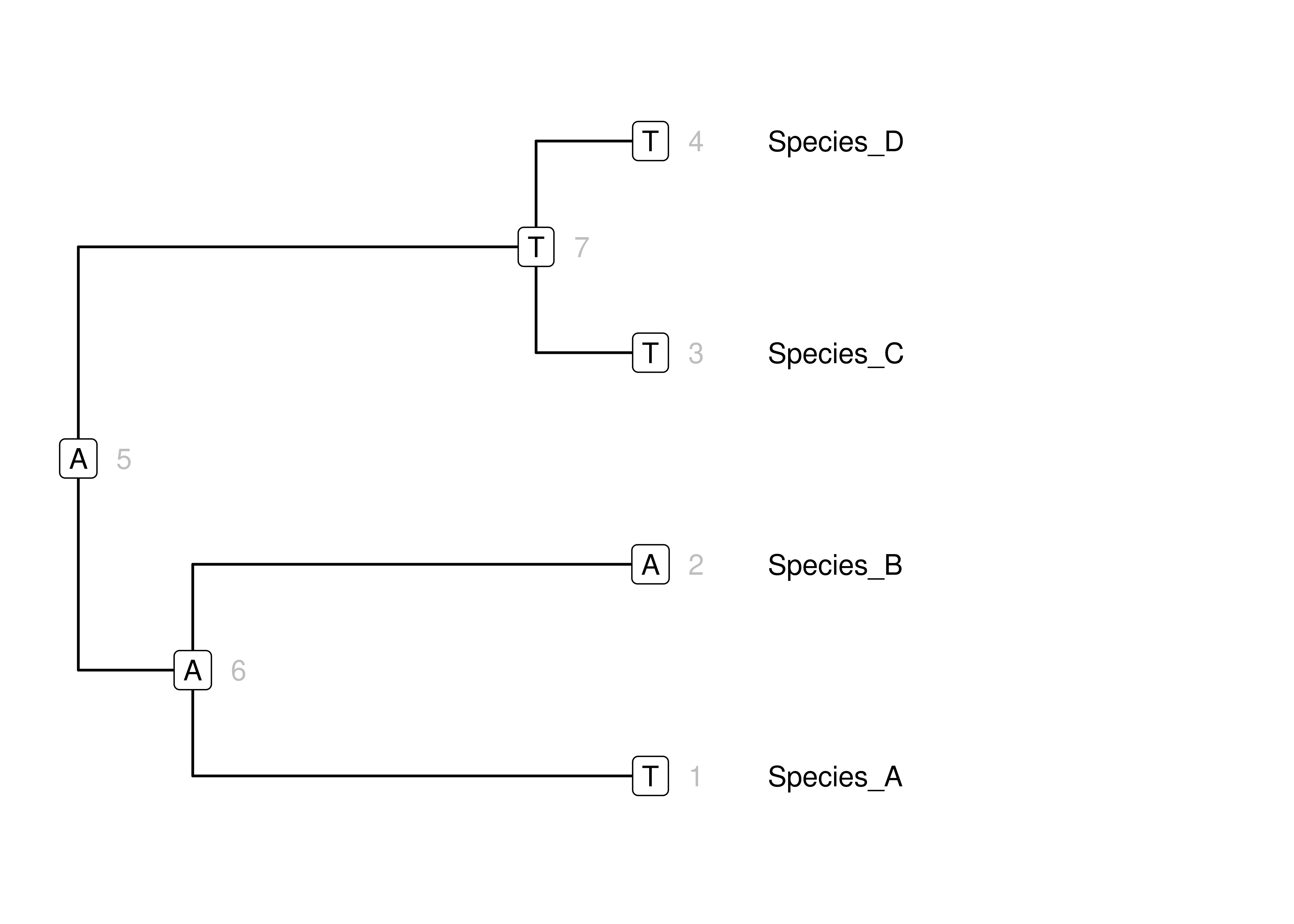
Figure 3.10: Simulation of states for a single DNA site on a simple tree according to our toy mammal model. Node numbers are in gray. Character states are in boxes at nodes. Branch lengths for this phylogram are in units of expected change.

This isn’t a big step from what we have already – once we have all the machinery to simulate along a single branch, we can just iterate that to simulate evolution along a whole tree.

Let’s start with the root of the tree (Figure 3.10, node 5). As in our simulations along single branches, we will pick the state from the equilibrium frequencies \(\boldsymbol{\Pi}\). That gives us the \(A\) at the root in Figure 3.10. The root node is the parent of two branches that descend from it. These two branches connect to node 6 (the most recent common ancestor of the clade (Species_A, Species_B)) and node 7 (the most recent common ancestor of the clade (Species_C, Species_D)). We simulate the states for these child nodes according to the state at the root (node 5), length \(t\) of each branch, and \(\mathbf{P}(t)\). In each case, this is just as when we simulated evolution along a single branch at a time, it is just that the branches share a parent node so the also share a parent state.

There are four more branches in this tree, each connected to a terminal node. One branch has parent node 6 and child node 1 (which is the Species_A terminal node). Now that we are not at the root things are a little different. Rather than draw the state for the parent node from \(\boldsymbol{\Pi}\), we just use the state that was simulated along the branch connecting node 5 to node 6. This state is \(A\). Now we simulate evolution along the branch connecting node 6 to node 1, given the state at node 6, length \(t\) of the branch, and \(\mathbf{P}(t)\). We then do the same for each of the other branches.

Data can be simulated on a tree of arbitrary size in this way. Just sample from \(\mathbf{P}(t)\) for the root state. Then traverse the tree from the root to each of the tips, simulating the state at each of the other internal nodes and finally the terminal nodes according to the states of their parents, branch length \(t\), and \(\mathbf{P}(t)\).

3.8 Scaling from a single site to multiple sites

So far we have considered evolution at a single DNA site across a whole phylogeny. Genomes have from thousands to billions of sites, though. Here we expand our simulations from a single nucleotide at a time to arbitrarily long DNA sequences.

How? With one simplifying assumption – that the evolution of each site is independent of the evolution at other sites. We just simulate one site at a time, and then stick all the results together into a sequence.

3.9 Concluding thoughts

Here we have built up the conceptual, mathematical, statistical, and computational machinery to simulating DNA evolution on a tree. Sequence simulation is useful for a variety of things, including generating datasets under known conditions to test tools. A major value, though, is to to think in a full explicit way about how you are modeling evolution. This probabilistic model framework is the exact same one we will use as we move to our next task, inferring phylogenies from sequence data.

3.10 Additional resources

• As a grad student, I learned much of what I present here from Swofford et al. (1996). This is such a lucid introduction to the likelihood of molecular sequence data on a phylogeny.

• My own thinking about presenting this material was heavily influenced by Paul Lewis’s wonderful lectures at the annual Workshop on Molecular Evolution at Woods Hole. Some of his lectures are now available online as part of the excellent Phylo Seminar at https://www.youtube.com/channel/UCbAzhfySv7nLCrNYqZvBSMg , starting with https://www.youtube.com/watch?v=1r4z0YJq580&t=2111s .

• A great introduction to continuous time models by John Huelsenbeck is available at https://revbayes.github.io/tutorials/dice/ .

References

Box, George EP. 1976. “Science and Statistics.” Journal of the American Statistical Association 71 (356): 791–99. https://doi.org/10.1080/01621459.1976.10480949.

Breiman, Leo et al. 2001. “Statistical Modeling: The Two Cultures (with Comments and a Rejoinder by the Author).” Statistical Science 16 (3): 199–231. https://projecteuclid.org/euclid.ss/1009213726.

Godfrey-Smith, Peter. 2013. Philosophy of Biology. Princeton University Press.

Jukes, TH, and CR Cantor. 1969. Evolution of Protein Molecules. Academic Press New York, NY. https://doi.org/10.1016/B978-1-4832-3211-9.50009-7.

Rosenberg, Michael S., Sankar Subramanian, and Sudhir Kumar. 2003. “Patterns of Transitional Mutation Biases Within and Among Mammalian Genomes.” Molecular Biology and Evolution 20 (6): 988–93. https://doi.org/10.1093/molbev/msg113.

Swofford, DL, GJ Olsen, PJ Waddell, and DM Hillis. 1996. Phylogenetic Inference. Edited by David M Hillis, Craig Moritz, Barbara K Mable, and Richard G Olmstead. Sinauer Associates Sunderland, MA.

Zapata, Felipe, Freya E Goetz, Stephen A Smith, Mark Howison, Stefan Siebert, Samuel H Church, Steven M Sanders, et al. 2015. “Phylogenomic Analyses Support Traditional Relationships Within Cnidaria.” PloS One 10 (10): e0139068.