Chapter 9 Additional character types
So far we have considered a single type of character data—DNA sequences. But there are many other types of characters that we would like to measure and analyze on phylogenies. These include morphology, protein sequences, protein structure, gene expression, physiological traits, and environmental tolerances. Different types of character data need to be handled in different ways. In particular, we need to be able to articulate explicit models for how each type of data evolves.
We can group character types based on shared features. Some data, such as the nucleotides of DNA, are discrete unordered values from a finite set \(\{A, C, G, T\}\) where the elements have no inherent ordering (e.g., \(C\) is not greater than \(A\), or less than \(T\)). Others have continuous values, such as mass or length, that fall in a particular order on the real number line (\(2.5\) is less than \(3.2\)). Still others, such as the number of bristles on a leg segment, have countable values represented with integers. These values are both discrete (there are no integers between \(3\) and \(4\)) and ordered (\(3\) is less than \(4\)). If we consider these different character types, it is clear not only that we measure and record them differently, but that the measurements themselves have different properties requiring different analysis methods. We could not, for example, construct a matrix like Equation (3.5) with rows and columns for every possible length in millimeters for flower petals.
Rather than approach each new character type in an ad hoc way, it is better to examine their general properties and explicitly consider how each character should be encoded and modeled. Specifying the character types is a critical aspect of how we articulate our ontological perspective (i.e., what organismal attributes exist, which are worth considering for the question at hand, and what the relation between them is). The character type your data correspond to is an intrinsic property that must be correctly identified. The criteria for making this evaluation and understanding its implications are part of measurement theory (Houle et al. 2011). This field sits at the intersection of math, statistics, and philosophy. It considers the relationships between measurements and the reality they represent, and clarifies what information the measurements contain. It examines which mathematical operations we can perform with them while preserving their meaning, and reveals what actual transformations those operations correspond to. With a name like “measurement theory”, you might assume that it is a dusty and boring annoyance that someone else needs to worry about, but it is actually a fascinating and grounding framework for understanding many of the central aspects of what we do in science.
| Scale type | Domain | Measurement type | Meaningful comparisons | Biological examples |
|---|---|---|---|---|
| Nominal | Any set of symbols | Discrete | Equivalence | Species, genes |
| Ordinal | Ordered symbols | Discrete | Order | Social dominance |
| Interval | Real numbers | Continuous | Order, differences | Dates, Malthusian fitness, relative temperature (arbitrary 0, e.g., Celsius and Fahrenheit) |
| Log-interval | Positive real numbers | Continuous | Order, ratios | Body size |
| Difference | Real numbers | Continuous | Order, differences | Log-transformed ratio-scale variables |
| Ratio | Positive real numbers | Continuous | Order, ratios, differences | Length, mass, duration, absolute temperature (e.g., Kelvin) |
| Absolute | Defined | Continuous | Any | Probability |
Because biological measurement developed pragmatically rather than from measurement theory, there are some differences in the nomenclature. What phylogenetic biologists call “character type” is referred to in measurement theory, and many other fields of science, as “scale type” (Table 9.1). Scale types vary in several ways. The Domain indicates the possible values. Phylogenetic methods differ most based on whether this domain is discrete or continuous, reflected here in the Measurement type column. Meaningful comparisons indicates comparisons that can be made between measurements of each scale type. Our comparisons should be constrained to respect the physical realities that our measurements represent, and measurement theory gives us formal tools to evaluate this. We should not, for example, compute the numerical difference between ordinal states, like social dominance ranks, because the actual physical or evolutionary distances between those ranks are unknown and unequal.
There are many types of organism measurements, and therefore state spaces and character types, that are addressed in a phylogenetic context. Here we consider some of the more frequently applied character types, i.e., scale types. Different scale types require different models of evolution.
9.1 Discrete character types
9.1.1 Nominal scale types
9.1.1.1 DNA nucleotides
Measurements of DNA sequences have 4 possible states, corresponding to each of the 4 nucleotides—\(\{A, C, G, T\}\). DNA data are discrete and unordered. Nucleotides are discrete because they have a set of distinct and separate states. They are unordered because changes don’t have to occur in a specific order; any state can change to any other state directly. In measurement theory terms, discrete unordered character types correspond to a nominal scale type.
9.1.1.2 Amino acids
Protein sequences are handled very similarly to DNA sequences, the character states just correspond to amino acids rather than to DNA nucleotides. They are discrete and unordered, and therefore on a nominal scale type. There are 20 possible states instead of 4, so the state space is larger. In principle this implies many more parameters, because the size of the rate matrix grows with the square of the number of states: a fully parameterized model of amino acid evolution has far more exchangeability parameters than a nucleotide model. In practice, however, these are rarely all estimated from the data at hand. Most protein analyses instead use empirical exchangeability matrices, such as JTT, WAG, or LG, whose values were estimated once from large databases of protein alignments and are then held fixed. As a result, the number of parameters actually estimated in a typical protein analysis can be comparable to, or even fewer than, in a nucleotide model, even though the underlying model describes a much larger state space.
There are a few reasons why protein sequences are often considered in phylogenetic analyses rather than the DNA sequences that encode them. One is that questions about protein evolution are best addressed with models that directly describe protein evolution. Another is that synonymous changes in protein-coding DNA sequences quickly saturate for more distant evolutionary comparisons. This means that much of the variation in DNA sequence has little information about phylogenetic relationships. Protein data can be more tractable to work with in this situation.
9.1.1.3 Codons
Since there are 4 possible DNA nucleotides and codons are 3 nucleotides long, there are \(4^3=64\) possible codons. Each one of these codons corresponds to a specific amino acid or stop codon. In some cases, it is most interesting to consider each of the 64 codons as a discrete character state. The models then have matrices with dimensions of \(64 \times 64\) (as opposed to 4 for nucleotides and 20 for amino acids).
9.1.1.4 Morphology
Direct analogs of the DNA sequence evolution models are often applied to discrete unordered morphological traits, such as the presence or absence of limbs (Harmon 2018, chap. 7). The most widely used of these is the Mk model (Lewis 2001), a \(k\)-state generalization of the Jukes-Cantor model in which all changes among \(k\) states occur at equal rates.
9.1.2 Ordinal scale types
Ordinal scale types include any kind of ranking, such as position in a social hierarchy (Houle et al. 2011, Table 1). They have an ordering, i.e., some values are larger than others. But there is no statement about the distance between the values. In a pecking order for chickens, \(1\) is dominant over \(2\) and \(2\) over \(3\), but that doesn’t indicate that there is a similar difference between \(1\) and \(2\) as there is between \(2\) and \(3\).
9.1.3 Discrete ordered characters
Discrete ordered characters are countable traits, such as the number of digits on a forelimb or the number of bristles on an arthropod appendage. Like ordinal characters they have an order, but unlike them the spacing between adjacent values is uniform and meaningful—the difference between 3 and 4 digits is the same as between 4 and 5. This uniform spacing is the defining feature of an interval scale (Houle et al. 2011, Table 1); because counts also have a true zero, however, they are strictly a ratio (or absolute) scale rather than a true interval scale. For modeling their evolution, what matters is that they are discrete and ordered with uniform steps between adjacent states.
Models for the evolution of discrete ordered characters can be described with the same language we used for nominal scale types. The rates for changes between non-adjacent values are just set to zero. \(5\), for example, will have a nonzero rate of change to \(6\) and \(4\) and a rate of zero to all other values. In this way, the rate matrix disallows instantaneous changes that skip intermediate values. For example, to evolve from a forelimb with 5 digits to one with 3 digits, the model requires that the character pass through an intermediate state of \(4\) digits.
Such a rate matrix describing the changes between 0-6 digits would have this form, if the rates were the same between all states:
\[\begin{equation} \mathbf{Q} = \left(\begin{array}{ccccccc} -\mu & \mu & 0 & 0 & 0 & 0 & 0 \\ \mu & -2\mu & \mu & 0 & 0 & 0 & 0 \\ 0 & \mu & -2\mu & \mu & 0 & 0 & 0 \\ 0 & 0 & \mu & -2\mu & \mu & 0 & 0 \\ 0 & 0 & 0 & \mu & -2\mu & \mu & 0 \\ 0 & 0 & 0 & 0 & \mu & -2\mu & \mu \\ 0 & 0 & 0 & 0 & 0 & \mu & -\mu \\ \end{array}\right) \end{equation}\]
9.2 Continuous data
Many characters, such as body mass, limb length, protein abundance, maximum swimming speed, and metabolic rate, can take values across a continuous range of real numbers. In phylogenetics, these traits are typically grouped under the umbrella of continuous character data, since values can vary smoothly and intermediate values are possible between any two observations.
Measurement theory distinguishes several different scale types (for example, interval and ratio scales) that may all have continuous values. In phylogenetic comparative analyses, these distinctions are usually ignored, and the traits are analyzed using a common set of evolutionary models. Sometimes, ignoring these distinctions has little practical impact, but sometimes it has major consequences.
9.2.1 Brownian motion
The most widely used model for continuous trait evolution on phylogenies is Brownian motion (BM) (Felsenstein 1973, 1985b). In this model, trait evolution is treated as a stochastic diffusion process along the branches of the phylogenetic tree. Trait values change through time by accumulating small random fluctuations. This can be conceptualized as infinitesimally small random steps along the number line, sometimes increasing the value and sometimes decreasing it.
Under BM, the expected change in the trait value is zero. This is not because there is no change under Brownian motion. It is because increases are just as common as decreases. If you run the same BM simulation many times and average the results, the average change across all of them will be zero. Each one, however, can be quite different from the original value and from each other (Figure 9.1). This is because the variance of the trait value increases linearly with time. The longer two lineages evolve independently, or the faster the change, the more different their trait values are expected to become.
Mathematically, Brownian motion can be written as
\[ dX(t) \sim \mathcal{N}(0, \sigma^2 dt) \]
where \(X(t)\) is the trait value at time \(t\), and \(\sigma^2\) is the diffusion rate, describing the amount of variance accumulated per unit of evolutionary time.
In phylogenetic applications of the Brownian motion model there are two primary parameters. One is the initial state, \(X_0\), which is the initial trait value. The other is the diffusion rate, \(\sigma^2\), which determines how quickly trait variance accumulates through time. Along a branch of length \(t\), the trait value at the descendant node is modeled as
\[ X_{\text{descendant}} \sim \mathcal{N}(X_{\text{ancestor}}, \sigma^2 t) \]
This means that the expected trait value at the end of the branch is equal to the value at the beginning of the branch, while the variance around that expectation grows in proportion to the branch length.
One reason BM is widely used is that it leads to a convenient statistical formulation. The vector of trait values observed at the tips of a phylogeny follows a multivariate normal distribution whose covariance structure is determined by the shared branch lengths of the tree. This property allows efficient likelihood-based and Bayesian inference.
The BM model is primarily used because it provides a mathematically tractable approximation to trait evolution. However, many biological traits do not actually evolve according to the assumptions of BM and violate the fundamental nature of the measurements being analyzed. For example, BM allows trait values to take any real number, including negative values. Many biological measurements, such as body mass or metabolic rate, are strictly positive. Sometimes these violations have little impact on inference, especially when the observed trait variation is far from biologically impossible values. In other cases, however, they can lead to misleading conclusions if the model poorly reflects the underlying evolutionary processes.
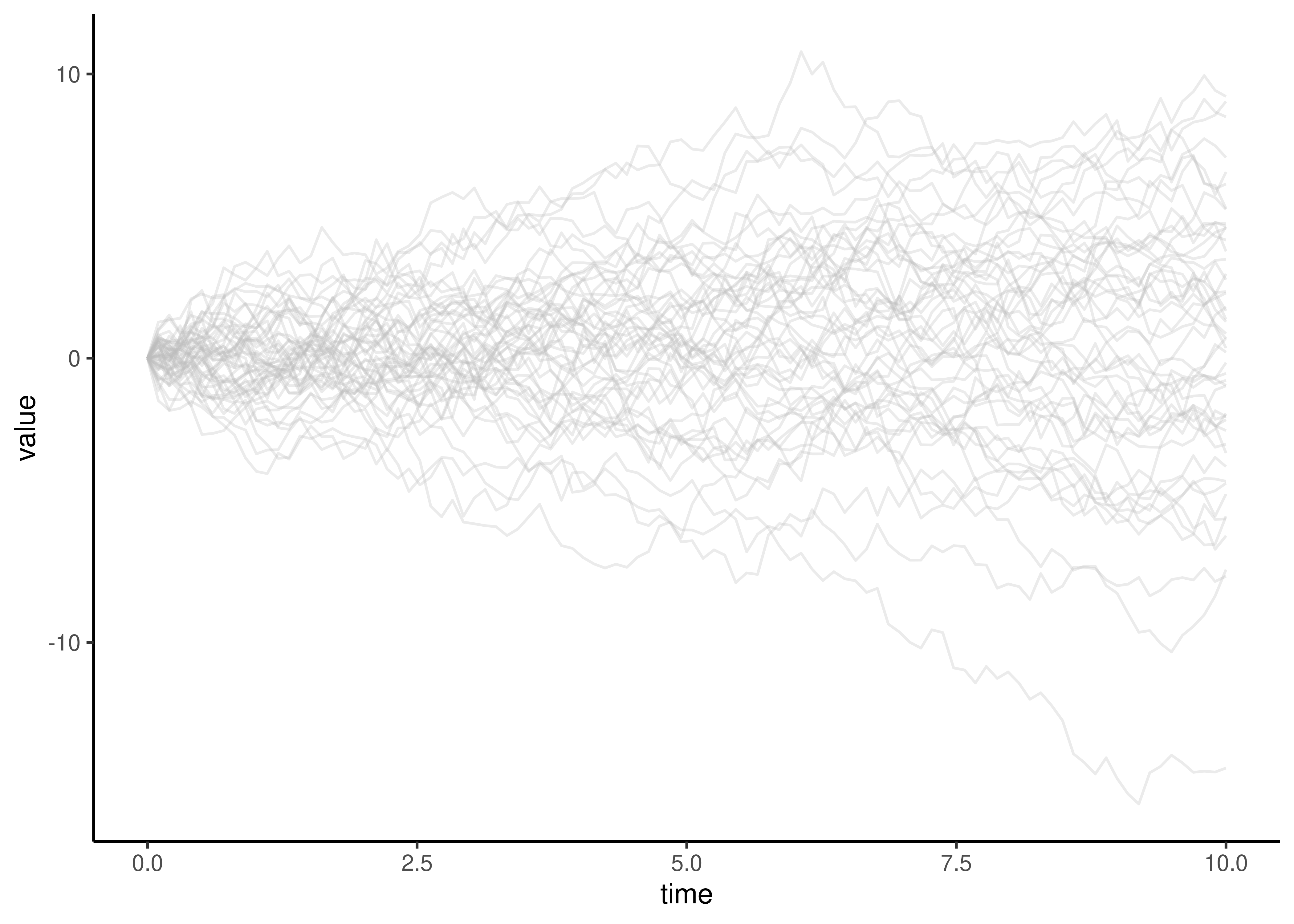
Figure 9.1: Multiple Brownian motion trajectories.
9.2.2 Ornstein–Uhlenbeck models
Brownian motion assumes that there is no preferred trait value or directional trend in evolution. In reality, traits are often subject to constraints, such as stabilizing selection or metabolic constraints, that lead values to stay near a particular optimum. The Ornstein–Uhlenbeck (OU) model is a common variation of Brownian motion that can accommodate these constraints (Hansen 1997; Butler and King 2004).
In the OU process, trait evolution is still driven by random fluctuations, but there is also a deterministic tendency for the trait value to move toward an optimum. The model can be written as
\[ dX(t) = \alpha(\theta - X(t))dt + \sigma dW(t) \]
where \(X(t)\) is the trait value at time \(t\), \(\theta\) is the value toward which the trait is drawn (often interpreted as an optimal trait value), \(\alpha\) describes the strength of attraction toward that value, and \(\sigma\) controls the magnitude of random fluctuations.
The OU model therefore includes both stochastic variation and a restoring force that pulls the trait toward an optimal value. When \(\alpha\) is large, trait values tend to remain close to the optimum. When \(\alpha\) is small, the restoring force is weak and trait values can wander more widely.
The Brownian motion model can be understood as a special case of the OU model. If the strength of attraction toward the optimum approaches zero (\(\alpha = 0\)), the restoring force disappears and the process reduces to pure Brownian motion. In this sense, OU models generalize Brownian motion by allowing processes in which trait values are pulled toward a central value rather than wandering freely.
It is important to be careful about the biological interpretation of these parameters. The OU model describes a statistical tendency for a trait to revert toward a central value; it does not, on its own, reveal why. Identifying \(\theta\) with an adaptive optimum, and a nonzero \(\alpha\) with stabilizing selection, is a biological interpretation that depends on the assumptions of the model (Hansen 1997; Butler and King 2004). A trait can appear to evolve under an OU process for reasons unrelated to adaptation, including bounds on the range of possible values, measurement error, or model misspecification. A good fit to an OU model is therefore consistent with stabilizing selection toward an optimum, but does not by itself demonstrate it, and inferring the underlying evolutionary process from the fit of a phylogenetic model alone is notoriously difficult (Uyeda et al. 2018). Distinguishing genuine adaptation from these alternatives generally requires additional evidence, such as a priori hypotheses about which lineages are expected to share an optimum.