Chapter 9 Phylogenies and time

Phylogenies consider the history, pattern, and process of evolution through time, so time is a critical feature of phylogenetic analyses. The specific considerations of time vary across analyses and studies, depending on the data available and the questions asked.

It is helpful to first think about how the elements of a phylogeny correspond to time. We will consider rooted trees, where the direction of time is specified and runs from the root to the tips. Each node occurs at a specific point in time, even if the specific timing is unknown. We will call this point in time the node age. There is often confusion about the description of relative time on phylogenies. I will describe the magnitude of age here as time before the present. A node minimum age is closer to the present (further forward in time) and a node with maximum age as further from the present (further back in time). A node is treated as a singular divergence event, and has no duration. This of course is an approximation of the actual biology of divergence, which can take place over a period of time as populations become increasingly isolated but gene flow may persist between them.

Each branch connects two nodes. In a rooted tree, we refer to the node closer to the root (or that is the root) as the parent node, and the node closer to the tips (or that is a tip) as the child node. The starting and ending times of the branch are set by the ages of the parent and child nodes. The duration of the branch is the difference in the ages of these nodes.

9.1 Measurements of time on trees

As discussed in Section 2.5, branch length can mean different things. It is up to the investigator to specify an branch length, and clearly communicate what it means. The three usual approaches are a cladogram (branch lengths are not specified and have no meaning), phylogram (branch lengths are the expected amount of evolutionary change in the traits used to infer the phylogeny), and chronogram, where branch lengths are in units of time.

9.1.1 Cladograms

Because branch lengths in a cladogram have no meaning, we cannot make absolute statements about time in a cladogram. This doesn’t mean, though, that we can’t say anything about time – we can still make some ordinal statements about the relative ages of nodes.

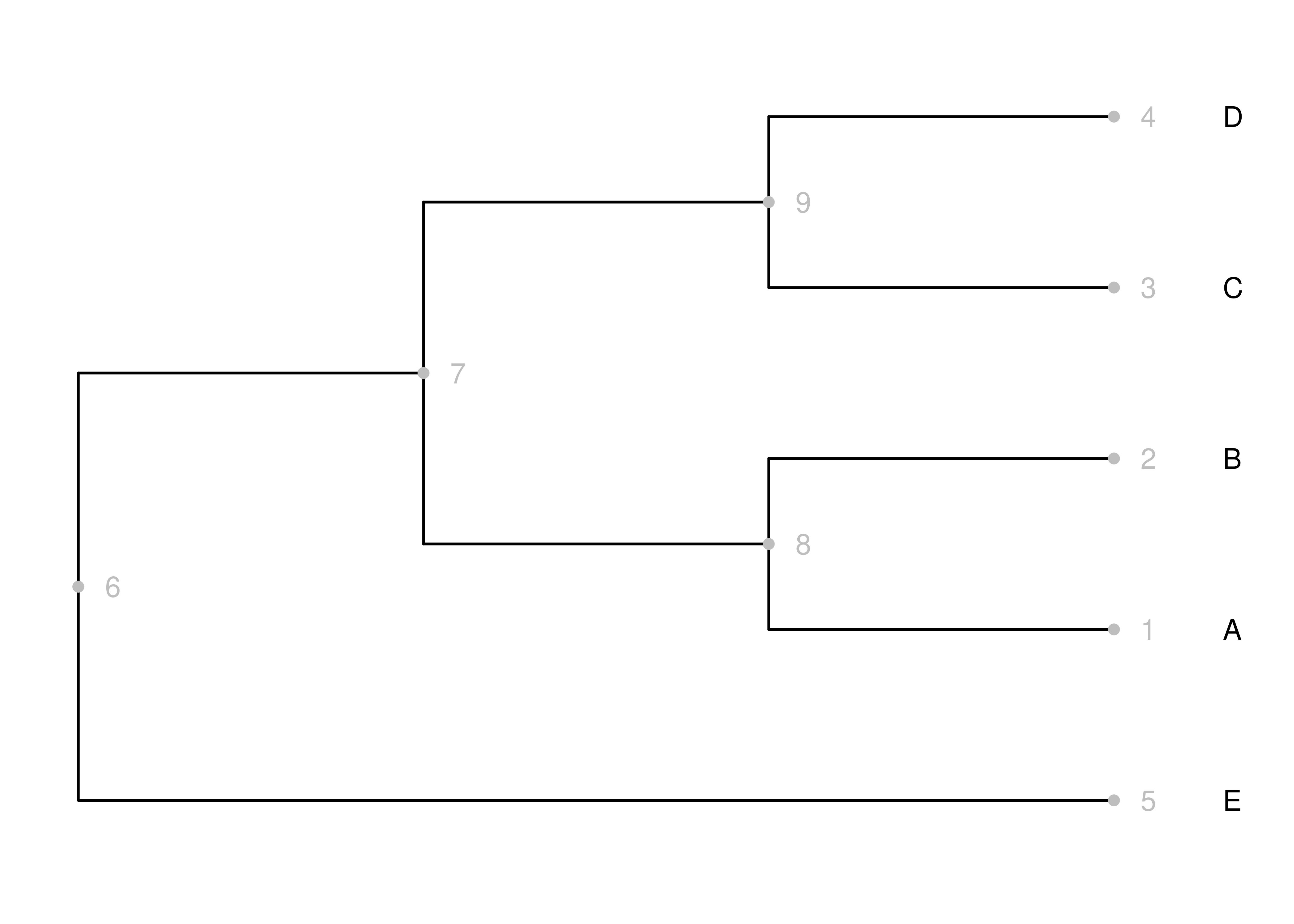
Figure 9.1: A cladogram. Nodes and node numbers are gray, and branches are black.

Take a look at the cladogram in Figure 9.1. Consider the red node numbers. The terminal nodes are numbered 1-5, and 6-9 are internal nodes. Of those, the root is node 6. Because the tree is rooted, we know that time proceeds from the root to the tips. If you consider two nodes, where one is descended from the other, then the node closer to the root is older. There are a variety of statements we could make based on this simple relationship, including:

• Node 6 is older than all other nodes in the phylogeny. This is tautological, since the root is by definition the oldest node.
• Node 7 is older than node 9. This is because 9 is descended form 7, and 7 is closer to the root.

We can’t make any relative assertions about the ages of nodes that aren’t descended from each other. For example, we have no idea of node 8 or node 9 is older.

In practice, these relative statements of age are often quite useful. For example, if Clade A is nested within Clade B, then we know that Clade A is younger than Clade B even if we don’t know the ages of any nodes. This may seem trivial, but it is implicit in many discussions of phylogenies.

Note that all of these assertions hold whether or not the tips have the same age. Tips can have different ages in a variety of scenarios, such as a real-time virus phylogeny sampled through the course of a phylogeny or if some tips are fossils.

9.1.2 Phylograms

Strictly speaking, the only assertions we can make about time on phylograms are those that we can also make on cladograms. This is because we can’t be certain of the relationships between time and branch length in the phylogram. If the rate of evolution changes in different regions of the tree, then branches of the same length would not represent time intervals of the same length. It is safest, then, to think of phylograms as cladograms when it comes to discussing time.

9.1.3 Chronograms

By definition, in a chronogram branch lengths are in units of time. The age of each node is fully specified. This has a couple implications for what we can say about time. We can make ordinal statements, as we did for cladograms and phylograms, but we can also make absolute statements about the interval of time that has elapsed between two nodes. We can also make statements about the relative ages of nodes that are not descended from each other.

9.2 Clock-like evolution

If the rate of evolution were uniform and did not vary in different lineages, then the branch lengths on the phylogram would be proportional to the elapsed time. We could convert from the phylogram to the chronogram just by dividing branch lengths by the rate of change. For example, if the branch lengths are in number of expected DNA substitutions, and the rate of evolutionary change is always 2 substitutions were million years, then dividing each branch length by 2 would give a chronogram where the units of branch length are millions of years. This is called clock-like evolution – changes in characters are like regular tics on a clock.

Real data are never this tidy, but when evolutionary rates are locally fairly uniform, then phylogram branch lengths will tend to be roughly proportional to the amount of time elapsed according to a locally adjusted clock. This is called a relaxed clock model.

9.3 Time calibration

The process of creating a chronogram is referred to as time calibration. There are a few parts to the process:

• Get a phylogram.
• Constrain the ages of some nodes using external evidence. This can be done by clamping them to a specific age or specifying a distribution of possible ages.
• Adjust branch lengths so that they are consistent with the ages of the clamped nodes, also adjusting the ages of the unclamped nodes as necessary. This is done by fitting clock-like models character change, and adjusting for local variations in rate.
• Assess robustness and confidence in the calibrated node ages and branch lengths.

There are multiply approaches to applying these steps. In the early days of the field, each step was done largely independently. A phylogram would be inferred, dates specified for some nodes, the branches would be stretched or shrunk to get them to fit the calibrations as closely as possible, and then the process would be repeated with slightly different input branch lengths or different calibrations to assess robustness.

The field has been moving toward more integrated approaches, including the simultaneous estimation of all of these features in a Bayesian framework. A Bayesian framework is a very natural way to incorporate diverse information about topology, branch lengths, and evolutionary rates. This has intuitive appeal – if the calibrations for two nodes indicate that they have a short branch between them, for example, then topologies that place these nodes together should be favored over other that do not. Constraints on node ages can be incorporated as priors, for example. Unconstrained nodes would have flat priors on age, and constrained nodes would have a sharp peak around a specific age.

9.3.1 Mathematical implications of age constraints

If all the tips are the same age, then the phylogeny is referred to as being ultrametric – each tip is the same distance from the root. An ultrametric tree is not necessarily a chronogram, though – some of the internal nodes may have ages that violate branch lengths proportional to time.

Clamping the ages of tips reduces the number of free parameters in our tree. The way to think about this is that the more information we have, the more constrained and specific our view of the world is. Before we clamp the tip ages, any tip can be any age and all the branches are free to have any length. The ultrametric tree is nested within this set of unconstrained possibilities. The tip ages, and therefore branch lengths, in this unconstrained tree can be selected so that they are ultrametric, but the vast majority of values will lead to trees that are not ultrametric. By clamping some values with added information that some nodes (tips, in this case) are the same age, we now are allowing only a constrained subset of trees and these require fewer parameters to describe.

It is easiest to think of this in terms of branch lengths, rather than node ages. From Section 2.3, we know that the number of branches in a tree is \(2n-2\), where \(n\) is the number of tips. This is because each of the \(n\) tip nodes has an branch leading to it, and each of the \(n-1\) internal nodes, with the exception of the root node, has an branch leading to it. So there are \(n-2\) branches that give rise to internal nodes. This is how we arrive at our \(n+n-2=2n-2\) branches in the phylogeny, each with their own length. In an ultrametric tree, by definition all the tips have the same age. That means that if you know the length of one of the branches leading to a tip node, you can calculate all the others. They have a deterministic relationship and are not free to vary independently. Rather than \(n\) branch lengths for the tips, we only have \(1\) tip branch length that is free to vary and we can calculate all the others so that the tip nodes have the same ages. This leaves us with \(1+n-2=n-1\) branch lengths that we need to estimate independently in our ultrametric tree.

9.3.2 Constraining node ages

All the tips sampled in the present day have the same age, and we can constrain them accordingly as described above. But to time calibrate our tree we need to constrain nodes at multiple time points. This is what allows us to establish rates that we can use to infer the ages of unconstrained nodes. There are two broad approaches to applying multiple constraints through time. The investigator can either constrain the ages of internal nodes (internal-node-calibrated phylogenies), in which all tips still have the same age, or some tips can be allowed to have ages that precede the present day (tip-calibrated phylogenies). We will illustrate both approaches with an example a study where we have 50 living organisms all sampled in the present day, and 10 fossils sampled across a range of times. We have a morphological character matrix for all, and can infer phylograms that we find to be consistent with a relaxed clock model.

In an internal-node-calibrated phylogeny, we would infer a phylogeny with all 60 taxa (fossil and extant), note the placement of the fossil taxa, and then infer the phylogeny with only the 50 extant taxa. We would constrain internal nodes so that they are no younger than the oldest fossil that is descended from them. We are considering a phylogeny of only extant taxa, but using the fossils to constrain the minimum age of the clades they belong to. In practice, it is also necessary to place maximum ages on some of the nodes to keep the time calibration from pushing everything way back in time. Given the incompleteness of the fossil record, this is not as straight forward as constraining the minimum age of a node. If we have a fossil we can assert that the clade that contains it can be no younger than that specimen, though it may be much older. But it is harder to assert a maximum age, given that we just might not have fossils for older organisms that existed in the clade. Applying maximum ages often relies on expertise and additional information, such as knowledge that a given land mass where the organisms are exclusively found did not exist before a particular time.

The internal-node-calibrated approach is simplest to implement in some respects, but has a variety of drawbacks. It doesn’t make good use of all the available information. By just setting minima on clade ages, it is discarding information about the branch lengths for the fossil taxa. If the branch giving rise to a fossil is long, then we might want to mush the minimum age for a clade much further back than the age of the fossil itself, for example. This approach also doesn’t work well has the fraction of fossil taxa increases in the analysis. For example, it wouldn’t work at all for a phylogeny comprised exclusively of fossil taxa.

In a tip-calibrated phylogeny, all taxa, fossil and extant, are included as tips in the phylogeny. The age of each tip is then constrained. Any tips from the present day are constrained to have the same present age, and fossil tips are constrained according to external information such as stratigraphy. A relaxed clock is then applied to infer the ages of unconstrained nodes, which also provides inferences of branch lengths.